InQuanto-NGLView

The InQuanto-NGLView extension provides basic utilities for visualizing chemical systems via the NGLView package. These utilities return NGL widgets which can be interactively viewed in a jupyter notebook. The functionality includes visualization of molecular structures, molecular fragmentation schemes, and molecular orbital isosurfaces.

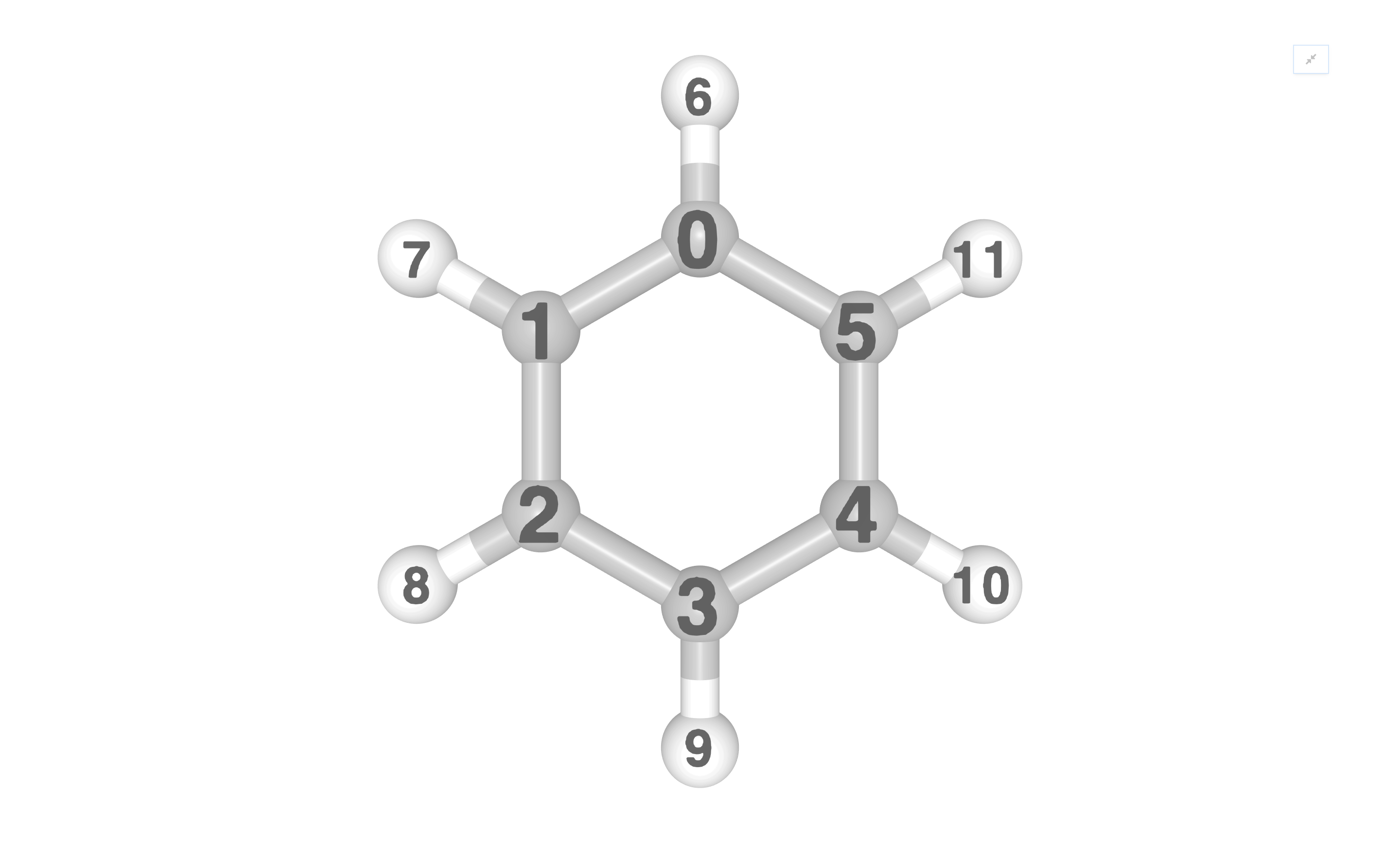
Visualizing Structures

The VisualizerNGL class is the central object of the InQuanto-NGLView extension. VisualizerNGL takes an InQuanto Geometry object as input, and produces an interactive NGLWidget with the visualize_molecule() method, visualizable in a jupyter notebook. See below for an example with molecular geometry:

from inquanto.geometries import GeometryMolecular
from inquanto.extensions.nglview import VisualizerNGL

xyz = [
    ['C', [ 0.0000000,  1.4113170, 0.0000000]],
    ['C', [ 1.2222370,  0.7056590, 0.0000000]],
    ['C', [ 1.2222370, -0.7056590, 0.0000000]],
    ['C', [ 0.0000000, -1.4113170, 0.0000000]],
    ['C', [-1.2222370, -0.7056590, 0.0000000]],
    ['C', [-1.2222370,  0.7056590, 0.0000000]],
    ['H', [ 0.0000000,  2.5070120, 0.0000000]],
    ['H', [ 2.1711360,  1.2535060, 0.0000000]],
    ['H', [ 2.1711360, -1.2535060, 0.0000000]],
    ['H', [ 0.0000000, -2.5070120, 0.0000000]],
    ['H', [-2.1711360, -1.2535060, 0.0000000]],
    ['H', [-2.1711360,  1.2535060, 0.0000000]]
]
c6h6_geom = GeometryMolecular(xyz)
visualizer = VisualizerNGL(c6h6_geom)
visualizer.visualize_molecule(atom_labels="index")

Note

Code snippets on this page generate interactive cells in a jupyter notebook. Static images are shown here for demonstration.

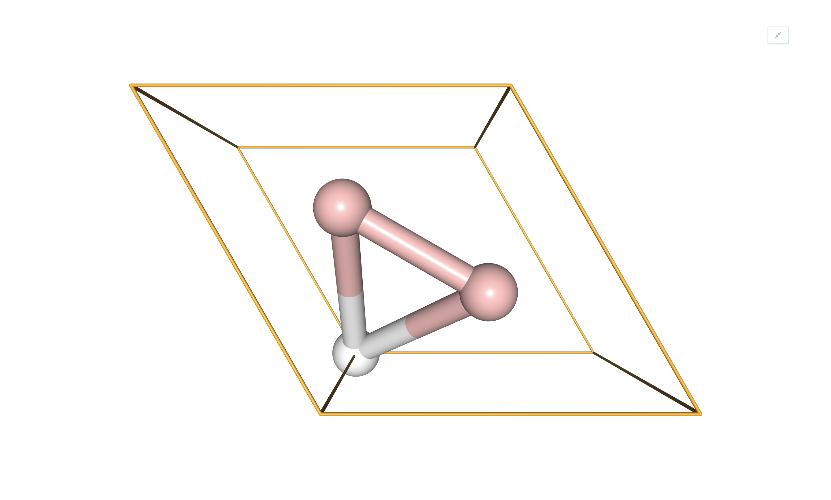
Similarly, periodic systems may be visualized by providing VisualizerNGL with a GeometryPeriodic object:

 from inquanto.extensions.nglview import VisualizerNGL
 from inquanto.geometries import GeometryPeriodic
 import numpy as np

 # AlB2 unit cell
 a=3.01 # lattice vectors in Angstroms
 c=3.27
 a, b, c = [
     np.array([a, 0, 0]),
     np.array([-a/2, a*np.sqrt(3)/2, 0]),
     np.array([0, 0, c])
 ]
 atoms = [
     ["Al", [0, 0, 0]],
     ["B", a/3 + b*2/3 + c/2],
     ["B", a*2/3 + b/3 + c/2]
 ]

alb2_geom = GeometryPeriodic(geometry=atoms, unit_cell=[a, b, c])
visualizer = VisualizerNGL(alb2_geom)
visualizer.visualize_unit_cell()

Visualizing Fragments

There are several fragmentation methods available in InQuanto; to visualize a fragmentation scheme defined in a GeometryMolecular object, use the visualize_fragmentation() method:

c6h6_geom.set_groups(
    "fragments",
    {
        "ch1": [0, 6],
        "ch2": [5, 11],
        "ch3": [4, 10],
        "ch4": [3, 9],
        "ch5": [2, 8],
        "ch6": [1, 7]
    }
)
visualizer.visualize_fragmentation("fragments", atom_labels="index")

Note

Visualizing fragments is not yet supported for periodic geometries.

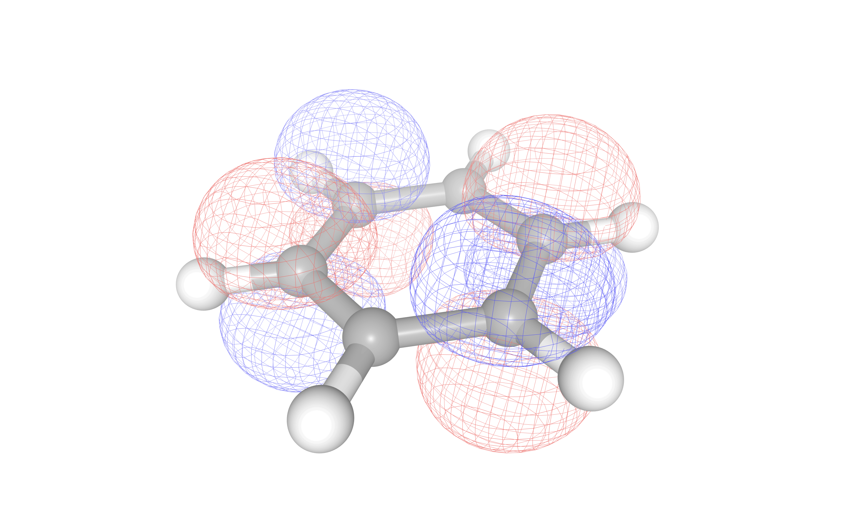
Visualizing Orbitals

To provide a visual aid in active space selection, molecular orbitals may be visualized with the visualize_orbitals() method. Orbital information must be provided in .cube format, which may be generated for molecular systems with the InQuanto-pyscf extension. In the example below, we generate the Hartree-Fock molecular orbitals for benzene in a minimal basis, and select the LUMO for visualisation.

from inquanto.extensions.pyscf import ChemistryDriverPySCFMolecularRHF

driver = ChemistryDriverPySCFMolecularRHF(geometry=c6h6_geom.xyz, basis="sto3g")

cube_orbitals=driver.get_cube_orbitals()
ngl_mos = [visualizer.visualize_orbitals(orb) for orb in cube_orbitals]
ngl_mos[21]

Finally we note that extended NGLView options can be exposed by rendering its graphical user interface (GUI) using the following option:

g = GeometryMolecular(xyz)
visualizer = VisualizerNGL(g)
visualizer.visualize_molecule().display(gui=True)