InQuanto-Phayes
The InQuanto-Phayes extension provides
an interface to phayes package that performs one flavor of Bayesian quantum phase estimation (QPE) introduced by K. Yamamoto, S. Duffield, Y. Kikuchi, and D. Muñoz Ramo [20]
using the QPE circuit protocols implemented into InQuanto.
See Iterative Phase Estimation Algorithms for the introduction to the other iterative QPE algorithms available in InQuanto.
The basic idea of Bayesian QPE is, in general, to update the prior distribution of the phase \(\phi\) by the Bayesian update rule
where \(P(\phi|m, k, \beta)\) and \(P(m|\phi, k, \beta)\) denote the posterior and likelihood, respectively.
The parameters \(k\) and \(\beta\) are generated for each update.
Bayesian QPE may be more efficient than the maximum likelihood approach, as the parameter selection can reflect the prior \(P(\phi)\).
The Bayesian QPE implemented as AlgorithmBayesianQPE has the following features:
Representation of the prior \(P(\phi)\) switches from Fourier to von Mises (wrapped Gaussian) automatically.
The parameters \(k\) and \(\beta\) are selected optimally from the prior.
See Ref. [20] for the technical details.
Below is a simple example demonstrating the usage of AlgorithmBayesianQPE.
As in the usage of the other iterative QPE algorithm classes, we prepare the
IterativePhaseEstimationStatevector object to handle the quantum circuits generated using the chemistry input.
from inquanto.express import get_system
from inquanto.mappings import QubitMappingJordanWigner
from inquanto.ansatzes import FermionSpaceAnsatzUCCSD
from inquanto.protocols import IterativePhaseEstimationStatevector

# Generate the spin Hamiltonian from the molecular Hamiltonian.
target_data = "h2_sto3g.h5"
fermion_hamiltonian, fermion_fock_space, fermion_state = get_system(target_data)
mapping = QubitMappingJordanWigner()
qubit_hamiltonian = mapping.operator_map(fermion_hamiltonian)

# Generate a list of qubit operators as exponents to be trotterized.
qubit_operator_list = qubit_hamiltonian.trotterize(trotter_number=1)

# The parameter `t` is physically recognized as the duration time in atomic units.
time = 0.25

# Preliminary calculated parameters.
ansatz_parameters = [-0.107, 0., 0.]

# Generate a non-symbolic ansatz.
ansatz = FermionSpaceAnsatzUCCSD(fermion_fock_space, fermion_state, mapping)
parameters = dict(zip(ansatz.state_symbols, ansatz_parameters))
state_prep = ansatz.subs(parameters)

# Construct the protocol to handle the iterative QPE circuits.
protocol = IterativePhaseEstimationStatevector(
).build(
    state=state_prep,
    evolution_operator_exponents=qubit_operator_list * time,
)
Then, we prepare the algorithm class.
import phayes
from inquanto.extensions.phayes import AlgorithmBayesianQPE
# This is needed for the numerical stability.
from jax import config
config.update("jax_enable_x64", True)

# Prepare the phayes state.
phayes_state = phayes.init(J=1000)
k_max = 300

algorithm = AlgorithmBayesianQPE(
    phayes_state=phayes_state,
    k_max=k_max,
).build(protocol)
phayes_state represents the prior distribution, either in the Fourier or von Mises representation.
k_max designates the cap of \(k\). The algorithm will not attempt to choose a higher value of k than this setting, in order to limit the maximum circuit depth.
In contrast to
AlgorithmInfoTheoryQPE
and
AlgorithmKitaevQPE,
AlgorithmBayesianQPE requires a feedback loop.
Driving such a feedback loop simply requires invoking the run() method as many times as the number of desired Bayesian updates.
import numpy
import matplotlib.pyplot as plt

# Number of Bayesian updates.
n_update = 50

# Execute the Bayesian QPE
for i in range(n_update):

    # Perform the single Bayesian update with `n_shots` of measurement samples.
    algorithm.run()

    # Show the current prior.
    if i % 10 == 0:
        mu, sigma = algorithm.final_value()
        mode = {True: 'Fourier', False: 'von Mises'}[bool(algorithm.phayes_state.fourier_mode)]
        print(f"i_update       = {i+1}")
        print(f"representation = {mode}")
        xmin = max(mu - 30 * sigma, 0)
        xmax = min(mu + 30 * sigma, 2)
        phi = numpy.linspace(xmin, xmax, 256)[:-1]
        plt.plot(-phi / time, algorithm.final_pdf(phi))
        plt.xlabel("$E$ / hartree")
        plt.ylabel("$P(E)$")
        plt.show()
i_update       = 1
representation = Fourier
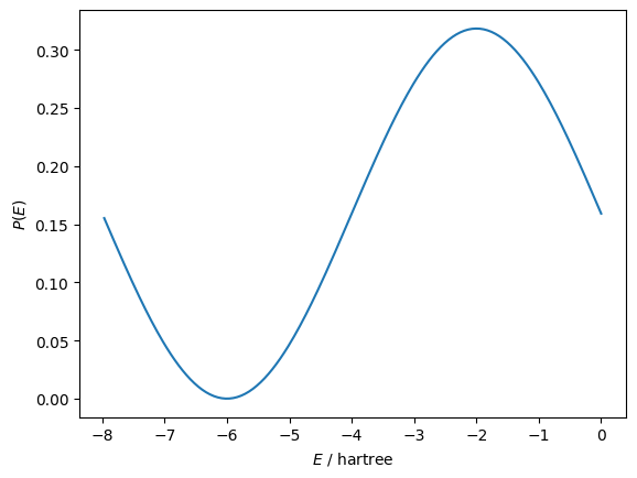
i_update       = 11
representation = Fourier
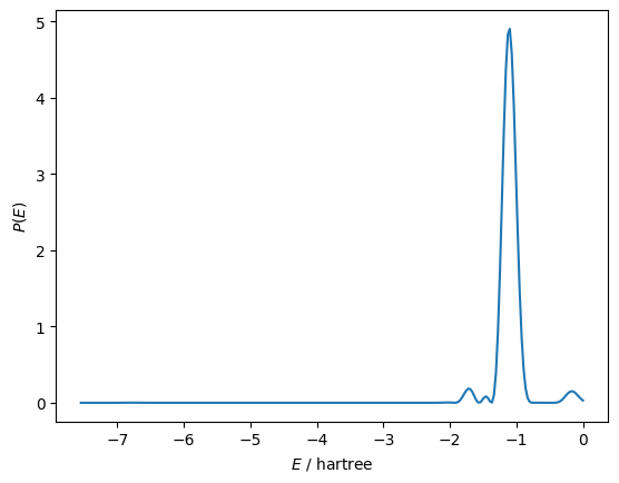
i_update       = 21
representation = Fourier
i_update       = 31
representation = von Mises
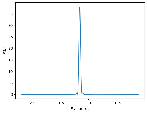
i_update       = 41
representation = von Mises
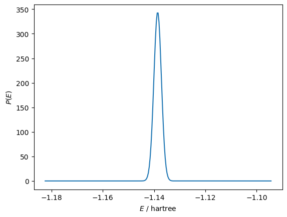
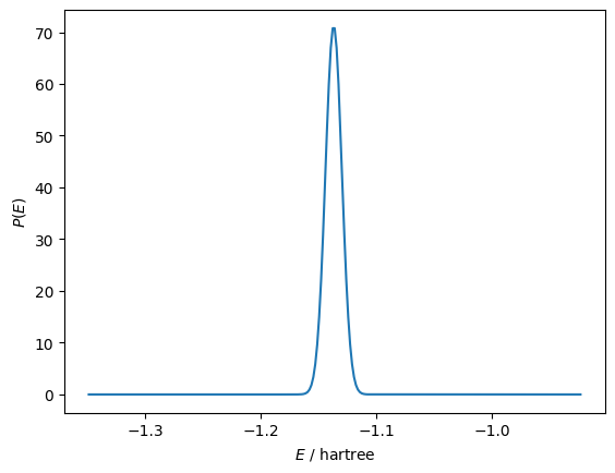
Note that the representation of the prior switches from Fourier to von Mises automatically. Now, the energy estimate is shown as a result of Bayesian QPE.
# Display the final results.
mu, sigma = algorithm.final_value()
energy_mu = -mu / time
energy_sigma = sigma / time
mode = {True: 'Fourier', False: 'von Mises'}[bool(algorithm.phayes_state.fourier_mode)]
print(f"i_update       = {i+1}")
print(f"Energy(mu)     = {energy_mu:10.6f} hartree")
print(f"Energy(sigma)  = {energy_sigma:10.6f} hartree")
print(f"Representation = {mode}")
i_update       = 50
Energy(mu)     =  -1.137974 hartree
Energy(sigma)  =   0.000995 hartree
Representation = von Mises