Density Matrix Embedding Theory

Density Matrix Embedding Theory (DMET) is a quantum embedding method developed to address the challenges of solving strongly correlated systems in quantum chemistry and condensed matter physics [58, 59]. This technique effectively partitions a large quantum system into smaller fragments and their corresponding environments, which allows for more manageable calculations.

The full DMET implementation involves nested iterations and fitting procedures to obtain a self-consistent one-body density matrix and an effective one-body correlation potential, which accounts for the correlation effects in the fragments. The accurate effective one-body correlation potential is found by solving the fragment problems using high-level classical or quantum methods and by comparing against results obtained through an effective Hamiltonian.

InQuanto supports various versions of DMET, including i) impurity DMET, which divides the total system into a single fragment and its environment; ii) one-shot DMET, which only optimizes the chemical potential; and iii) full DMET, which utilizes a chemical potential and an arbitrary parameterization of the one-body correlation potential.

Typically prior to the embedding algorithm one needs to generate a Hamiltonian with a localized and orthonormal basis or atomic orbitals, in which spatial fragments can be specified. In addition, DMET requires an initial density matrix of the total system, which is usually the one-electron reduced density matrix (1-RDM), calculated with a lower level quantum chemical method, in the respective localized basis. In InQuanto this can be computed by an extension chemistry driver. Moreover, traditional chemistry methods can also be used as high level fragment solvers and inquanto-pyscf extension has a number of fragment solvers for the user to combine.

Impurity DMET

InQuanto’s impurity DMET method is the simplest of its kind because it only deals with one selected fragment of a larger system. The initial 1-RDM in the localized basis is used to find new orbitals (fragment orbitals) such that the environment block of the 1-RDM in the basis of the new orbitals becomes diagonal. The Schmidt decomposition and DMET guarantee that the number of fractional diagonal elements in the environment block will be bounded by the size of the fragment block. Those orbitals associated with fractional diagonals in the environment block are called the bath orbitals, and the remaining orbitals, which are associated with integer diagonal elements (i.e., fully occupied or unoccupied orbitals), are called environment orbitals.

In the new orbitals, the active space is chosen as the orbitals for the fragment and the bath part, and the fragment calculation is reduced to the active space Hamiltonian, which without the constant terms takes the (fermionic) form of:

(102)\[\begin{split}\hat{H}_{\text{emb}} = \sum_{pq \in A \cup B} ( h_{pq} + \sum_{rs \in E}( (pq|rs) - (ps|rq) ) \Gamma^{\text{env}}_{rs}) \hat{a}_p^\dagger \hat{a}_q \\ + \frac{1}{2} \sum_{pqrs \in A \cup B} (pq|rs) \hat{a}^\dagger_p \hat{a}_r^\dagger \hat{a}_{s} \hat{a}_q\end{split}\]

where \(A\) is the set of fragment orbitals, \(B\) is the set of bath orbitals, \(E = \overline{A \cup B}\) is the set of environment orbitals, \(\hat{a}^\dagger\) and \(\hat{a}\) are fermionic creation and annihilation operators in the fragment basis, respectively, and \(\Gamma^{\text{env}}_{rs}\) is the 1-RDM constructed from the fully occupied environment orbitals only.

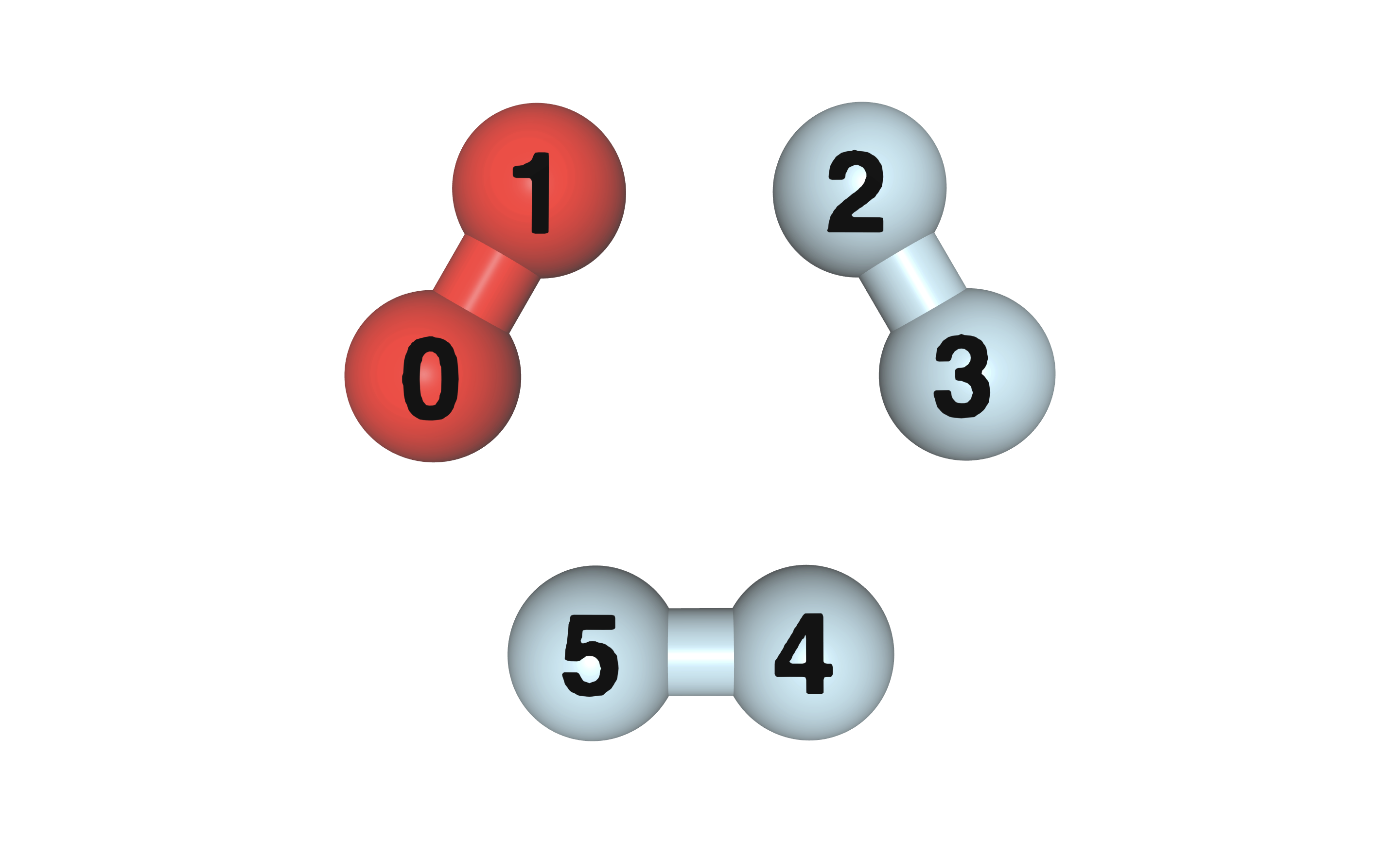
../_images/dmet3H2.png — Fig. 25 Three H₂ molecules in a ring arrangement, the H₂ molecule in red color is selected as the fragment.

To demonstrate a simple calculation, the following example will load the necessary inputs for a 6-atom H ring from the express module. The 6 atoms are arranged as 3 pairs of H₂ molecules forming a hexagon, with the atoms indexed as shown in Fig. 25. The Hamiltonian and the Hartree-Fock (HF) 1-RDM are computed with the STO3G basis set and with the Löwdin transformation. This results in 6 spatial orbitals, one for each hydrogen atom. The Löwdin transformation ensures that the spatial orbitals are localized and orthonormal, making them suitable for DMET calculations. After acquiring the input data, the impurity DMET method can be initialized:

from inquanto.express import load_h5
from inquanto.embeddings import ImpurityDMETROHF

h2_3_ring_sto3g = load_h5("h2_3_ring_sto3g.h5", as_tuple=True)

dmet = ImpurityDMETROHF(
    h2_3_ring_sto3g.hamiltonian_operator_lowdin, h2_3_ring_sto3g.one_body_rdm_hf_lowdin
)

The impurity DMET method class ImpurityDMETROHF is initialized with the Hamiltonian operator and the 1-RDM in the localized basis. The name of the class indicates that this method assumes the Hamiltonian operator and the 1-RDM are spin-restricted.

In this specific example, we select the first H₂ molecule as a fragment, which consists of the first two consecutive H atoms in the ring. The fragment and its bath will be treated with a high-level solver. In InQuanto, the fragment is defined by a spatial orbital mask and a fragment solver as follows:

from numpy import array
mask = array([True, True, False, False, False, False])

from inquanto.embeddings import ImpurityDMETROHFFragmentED
fragment = ImpurityDMETROHFFragmentED(dmet, mask)

The mask is a boolean array with a length equal to the number of localized spatial orbitals. The True values in the mask select the indices of the localized spatial orbitals that belong to the fragment. The elaborate classname ImpurityDMETROHFFragmentED defines a high-level solver for the fragment, which is responsible for calculating the ground state of the fragment+bath system during the DMET procedure. In this specific example, the solver employs an exact diagonalization method.

To perform the DMET calculation, call the run method:

result = dmet.run(fragment)

The advantage of this simple single-fragment version of DMET is its variational nature, with no iterative part outside the solvers, and this makes it more suitable for present noisy quantum algorithms.

To include more than one fragment in the DMET method, use the DMETRHF class, which is described in the next subsection.

One-shot DMET

One-shot DMET allows a total system to be decomposed into fragments, and each fragment will have its own bath and will be treated with its own fragment solver. The method introduces a global chemical potential as a self-consistency parameter to ensure that fractional charges on the fragments eventually sum up exactly to the total charge of the system. The Hamiltonian of a fragment plus bath (embedding system), which the fragment solver needs to handle, is

(103)\[\hat{H}_{\text{emb}}(\mu) = \hat{H}_{\text{emb}} - \mu \sum_{p \in A} \hat{a}^\dagger_{p} \hat{a}_p\]

where \(\mu\) is the introduced global chemical potential. The value of \(\mu\) is determined by the global constraint

(104)\[\sum_{f} \langle\Psi_{f}(\mu) | \hat{N}_{f} | \Psi_{f}(\mu)\rangle = N_{\text{tot}},\]

where \(\Psi_{f}(\mu)\) is the ground state of fragment \(f\), calculated by a high-level method, \(\hat{N}_{f}=\sum_{p \in A_f} \hat{a}^\dagger_{p} \hat{a}_p\) is the particle number operator of fragment \(f\) and \(N_{\text{tot}}\) is the total number of electrons in the system. In InQuanto, this constraint is satisfied by employing an iterative solver.

The ground state energy of the total system is calculated from the individual ground state calculations of the fragments based on the democratic mixing [60] of density matrix elements, and to avoid double counting of the environmental terms, the fragment’s energy contribution to the total energy is calculated with the fragment energy operator and not the Hamiltonian:

(105)\[\begin{split}\hat{E}_{\text{emb}} = \sum_{p \in A} \bigg( \sum_{q \in A \cup B} \bigg(h_{pq} + \frac{\sum_{rs \in E} [(pq|rs) - (ps|rq)] \Gamma^{\text{env}}_{rs}}{2}\bigg) \hat{a}^{\dagger}_p \hat{a}_q \\ + \frac12 \sum_{qrs \in A \cup B} (pq|rs) \hat{a}^\dagger_p \hat{a}^\dagger_r \hat{a}_s \hat{a}_q \bigg).\end{split}\]

The total electronic energy is calculated as a sum of the fragment contributions, \(\sum_{f} \langle\Psi_{f}(\mu) | \hat{E}_{\text{emb},f} | \Psi_{f}(\mu)\rangle\), where \(\hat{E}_{\text{emb},f}\) denotes the fragment energy operator from the equation above for fragment \(f\), and \(\Psi_{f}\) denotes the high level solution for fragment \(f\).

To demonstrate the one-shot DMET on the 6-atom ring toy system, we need to instantiate the class DMETRHF first:

from inquanto.embeddings import DMETRHF

h2_3_ring_sto3g = load_h5("h2_3_ring_sto3g.h5", as_tuple=True)

dmet = DMETRHF(
    h2_3_ring_sto3g.hamiltonian_operator_lowdin, h2_3_ring_sto3g.one_body_rdm_hf_lowdin
)

The fragments are similarly defined as in the impurity DMET case. In this particular example, we decompose the total system into three H₂ fragments and use a black-box statevector (i.e. ideal classical simulation) fragment solver DMETRHFFragmentUCCSDVQE which utilizes the UCCSD ansatz and optimises the ansatz parameters using VQE:

mask1 = array([True, True, False, False, False, False])
mask2 = array([False, False, True, True, False, False])
mask3 = array([False, False, False, False, True, True])

from inquanto.embeddings import DMETRHFFragmentUCCSDVQE
from pytket.extensions.qiskit import AerStateBackend

backend=AerStateBackend()
fragment1 = DMETRHFFragmentUCCSDVQE(dmet, mask1, backend=backend)
fragment2 = DMETRHFFragmentUCCSDVQE(dmet, mask2, backend=backend)
fragment3 = DMETRHFFragmentUCCSDVQE(dmet, mask3, backend=backend)

fragments = [fragment1, fragment2, fragment3]

It is essential that the set of fragments completely covers the entire system. To run the one-shot DMET procedure, call the run method:

result = dmet.run(fragments)

Full DMET with correlation matrix

In the full DMET simulation, the effect of a one-body correlation potential from the environment is also added to the embedding Hamiltonian, as follows:

(106)\[\hat{H}_{\text{emb}}(\mu, C) = \hat{H}_{\text{emb}}(\mu) + V_{\text{emb}}(\sum_{p,q \notin A} C_{pq} \hat{a}^\dagger_{p} \hat{a}_q)\]

By computing the ground state of this Hamiltonian with a high-level method, an accurate 1-RDM, \(\Gamma^A_{pq}\), is obtained for the fragment. In turn, the full DMET method finds the effective one-body correlation for the fragment, that is, \(C_{pq} \hat{a}^\dagger_{p} \hat{a}_q\) for \(p,q \in A\) such that a mean-field (MF) solution 1-RDM, \(\Gamma^{A,\text{MF}}_{pq}\), of

(107)\[\hat{H}_{\text{emb}}(\mu, C)' = \hat{H}_{\text{emb}}(\mu) + V_{\text{emb}}(\sum_{p,q \notin A} C_{pq} \hat{a}^\dagger_{p} \hat{a}_q) + \sum_{p,q \in A} C_{pq} \hat{a}^\dagger_{p} \hat{a}_q\]

minimally differs from \(\Gamma^A_{pq}\), that is, \(|\Gamma^A_{pq}-\Gamma^{A,\text{MF}}_{pq}|\) is minimum. In practice, since the mean-field solution is usually already available for \(\hat{H}_{\text{emb}}(\mu, C)\), the correlation potential is added to its effective mean-field version, and this is solved instead of \(\hat{H}_{\text{emb}}(\mu, C)'\). DMET performs this procedure for every fragment and, with the updated values of \(\mu\) and \(C_{pq}\), repeats the procedure again until self-consistency is reached. At this point, the fragment energies are computed to calculate the total electronic energy.

The technical difference from one-shot DMET is that we also need to input a parameterization for the correlation potential \(C_{pq}\). The DMETRHF class can take this parameterized correlation potential matrix, in pattern matrix format, as a constructor parameter. For example, for the 6-atom H ring, if we have two independent parameters in the correlation potential matrix, we prepare a pattern matrix that defines where the two independent parameters are:

import numpy

pattern = numpy.array(
    [
        [None, 0, None, None, None, None],
        [0, None, None, None, None, None],
        [None, None, None, 1, None, None],
        [None, None, 1, None, None, None],
        [None, None, None, None, None, 0],
        [None, None, None, None, 0, None],
    ]
)

In this pattern matrix, the 0 and 1 indices refer to the first and second independent parameters. The None matrix elements in the pattern indicate that the corresponding values of \(C_{pq}\) will be kept zero. A parameter can appear in more than one place in the pattern matrix, which could reflect the symmetry of the system. In this example, there are three 2-atom fragments, which are all equivalent. Therefore, due to symmetry, we could use just a single independent parameter and replace the index 1 with index 0 in the pattern matrix. However, to demonstrate the use of independent parameters, in this example we introduce this symmetry-breaking parameterization; i.e. we choose a parameterization that is not required to follow the system’s symmetry. At the end of the DMET run, we expect that the two independent parameters converge to the same value.

To perform the full DMET, one should call:

energy, chemical_potential, parameters = dmet.run(fragments, pattern)

Custom fragments

When running a hybrid quantum-classical algorithm as part of the DMET method flow, it is important to have the ability to create custom fragment solver classes. There are various ansatzes and strategies for performing a VQE simulation. In InQuanto, only one pre-implemented VQE fragment solver, DMETRHFFragmentUCCSDVQE, is provided. To ensure greater versatility, we offer an easy way to define a custom fragment solver. To do this, one can subclass the DMETRHFFragmentActive, which requires implementing the solve_active(...) method. This method assumes that the Hamiltonian, Fragment Energy operator and other arguments are only provided for the active space, which can be specified when the fragment solver is constructed. The mandatory return values are the expectation value of the Hamiltonian and the Fragment Energy operator with the ground state (energy and fragment_energy below), as well as the 1-RDM of the ground state:

class MyFragment(DMETRHFFragmentActive):

    def solve_active(
         self,
         hamiltonian_operator: ChemistryRestrictedIntegralOperator,
         fragment_energy_operator: ChemistryRestrictedIntegralOperator,
         fermion_space: FermionSpace,
         fermion_state: FermionState,
    ):

        # ... your VQE solution ...

        return energy, fragment_energy, vqe_rdm1

You can find complete executable examples in the examples/embeddings folder. The active space can be specified with the frozen argument at instantiation, by listing the HF orbital indices for the embedding system. One should be aware that since the embedding system is composed of the fragment and bath orbitals, and the number of bath orbitals is at most the number of fragment orbitals, the maximum number of orbitals is twice the number of fragment orbitals. In the 6-atom ring example, the H₂ fragment has 2 spatial orbitals, therefore the total number of orbitals in a fragment solver is 4, allowing us to freeze, for example, the lowest and the highest energy HF orbitals with indices 0 and 3, respectively:

fr = MyFragment(dmet, mask, frozen=[0, 3])

The fragment solvers for the impurity DMET are simpler because there is only a single fragment, so it is not necessary to calculate the fragment energy. In this case, it is recommended to subclass the ImpurityDMETROHFFragmentActive to make a custom class and implement the solve_active(...) method.

class MyFragment(ImpurityDMETROHFFragmentActive):

    def solve_active(
        self,
        hamiltonian_operator: ChemistryRestrictedIntegralOperator,
        fermion_space: FermionSpace,
        fermion_state: FermionState,
    ):

        # ... your VQE solution ...

        return energy

The mandatory return value is the ground state energy of the embedding system. Again, there are complete running examples in the examples/embeddings folder.

DMET for model systems and other Hamiltonians

InQuanto’s DMET embedding methods are designed to be flexible and compatible with various types of Hamiltonians as long as they meet specific requirements:

The Hamiltonian must be in a localized orthonormal basis.
The Hamiltonian type should be ChemistryRestrictedIntegralOperator.

With these requirements met, you can use DMET-based embedding methods with Hamiltonians from various sources, for example:

Periodic Systems: You can construct a Hamiltonian for a periodic system and use it with the API, enabling the study of crystalline or other periodic structures.
Model Hamiltonians: Using the Hubbard driver, you can generate model Hamiltonians that can be used with the DMET-based embedding methods API. This capability allows you to explore simplified systems and gain insights into more complex ones.
COSMO-generated Hamiltonians: By using the inquanto-pyscf extension, you can generate Hamiltonians with COSMO and use them with the API of DMET-based embedding methods. This feature enables the study of solvent effects and other environmental influences on your system of interest.