Protocols for expectation values

Shot-based protocols for measuring expectation values use quantum circuits to evaluate expressions of the form:

(38)\[\langle\Psi(\boldsymbol{\theta})|\hat{O}|\Psi(\boldsymbol{\theta})\rangle = \sum_{i} h_{i} \langle\Psi(\boldsymbol{\theta})| P_i |\Psi(\boldsymbol{\theta})\rangle.\]

where \(|\Psi(\boldsymbol{\theta})\rangle\) is a parameterized ansatz and the operator kernel is expressed as a linear combination of Pauli strings i.e. a QubitOperator:

(39)\[\hat{O} = \sum_i h_i P_i\]

This operator might be a chemistry Hamiltonian, obtained by means of Jordan-Wigner or Brayvi-Kitaev mapping for example.

Each term in (38) is an expectation value of a Pauli string. Each of these terms may be measured by preparing the ansatz of choice and appending some measurement gadget. InQuanto provides two methods to measure expectation values in this way, which are discussed below. The first is the PauliAveraging protocol, which directly operates on and measures the state register, and uses measurement reduction. The second is the HadamardTest protocol, which uses an ancilla qubit for measurement.

Note

All protocols discussed here are designed to handle a single input ansatz \(|\Psi(\boldsymbol{\theta})\rangle\). To efficiently generate circuits for expectation values with a range of input states, use the ProtocolList class, or build_protocols_from() method to group supported protocols together.

PauliAveraging

The PauliAveraging protocol uses Pauli partitioning to collect operator terms into simultaneously measurable sets. Consider the example below for minimal basis \(\text{H}_2\) with a simple ansatz:

from inquanto.express import load_h5
from sympy import sympify
from inquanto.operators import QubitOperator,QubitOperatorList
from inquanto.states import QubitState
from inquanto.ansatzes import TrotterAnsatz
from inquanto.computables import ExpectationValue
from inquanto.protocols import PauliAveraging
from pytket.extensions.qiskit import AerBackend
from pytket.partition import PauliPartitionStrat

h2 = load_h5("h2_sto3g.h5", as_tuple=True)
hamiltonian = h2.hamiltonian_operator.qubit_encode()
print("Number of terms in hamiltonian: ", len(hamiltonian))

theta = sympify("theta")
exponents = QubitOperatorList(QubitOperator("Y0 X1 X2 X3", 1j), theta)
reference = QubitState([1, 1, 0, 0])
ansatz = TrotterAnsatz(exponents, reference)

energy = ExpectationValue(ansatz, hamiltonian)

protocol = PauliAveraging(
   backend=AerBackend(),
   shots_per_circuit=1000,
   pauli_partition_strategy=PauliPartitionStrat.CommutingSets
)
protocol.build_from({theta: -0.111}, energy)
protocol.run()

print("Number of circuits: ", protocol.n_circuit)

energy.evaluate(protocol.get_evaluator())

Number of terms in hamiltonian:  15
Number of circuits:  2

-1.129918760208275

The full qubit-encoded hamiltonian is given by:

(40)\[\begin{split}\hat{H} = h_0 + h_1 Z_0 + h_2 Z_2 + h_3 Z_1 + h_4 Z_3\\ + h_5 Z_0Z_2 + h_6 Z_1Z_3 + h_7 Z_0Z_1 + h_8 Z_1Z_2\\ + h_9 Y_0X_1X_2Y_3 + h_{10} X_0X_1Y_2Y_3 + h_{11} Y_0Y_1X_2X_3\\ + h_{12} X_0Y_1Y_2X_3 + h_{13} Z_0Z_3 + h_{14} Z_2Z3\end{split}\]

The ExpectationValue computable for the total energy is provided to the protocol via the build_from() method, along with numerical values for any ansatz parameters (theta above). The Hamiltonian terms are grouped into two commuting sets, corresponding to two measurement circuits:

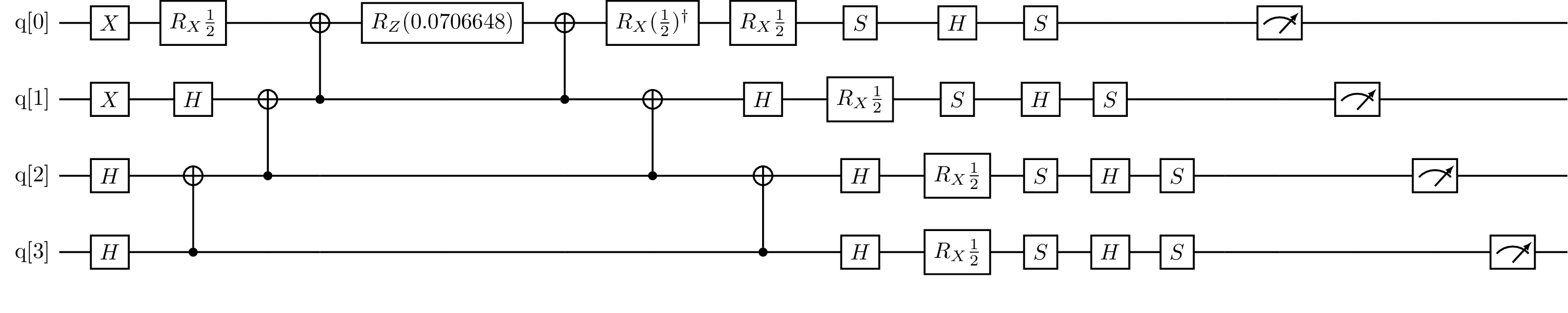
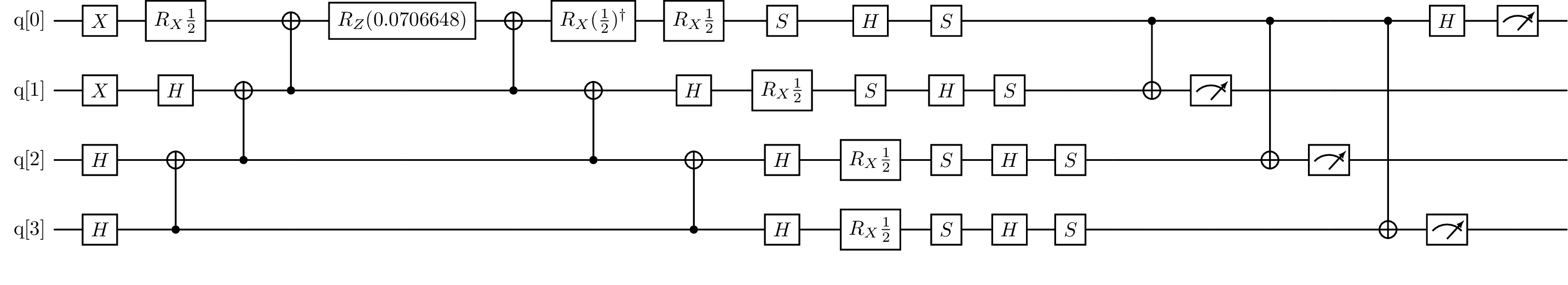
Fig. 7 Measurement circuits generated by the PauliAveraging example above.

The first circuit measures the expectation value of the individual Z terms in the Hamiltonian. The second circuit measures the remainder. The final expectation value of the operator is then the sum over the product of Pauli term weights \(h_i\) with the measured expectations \(\langle P_i \rangle\).

In general, the measurement circuits generated by PauliAveraging take the form:

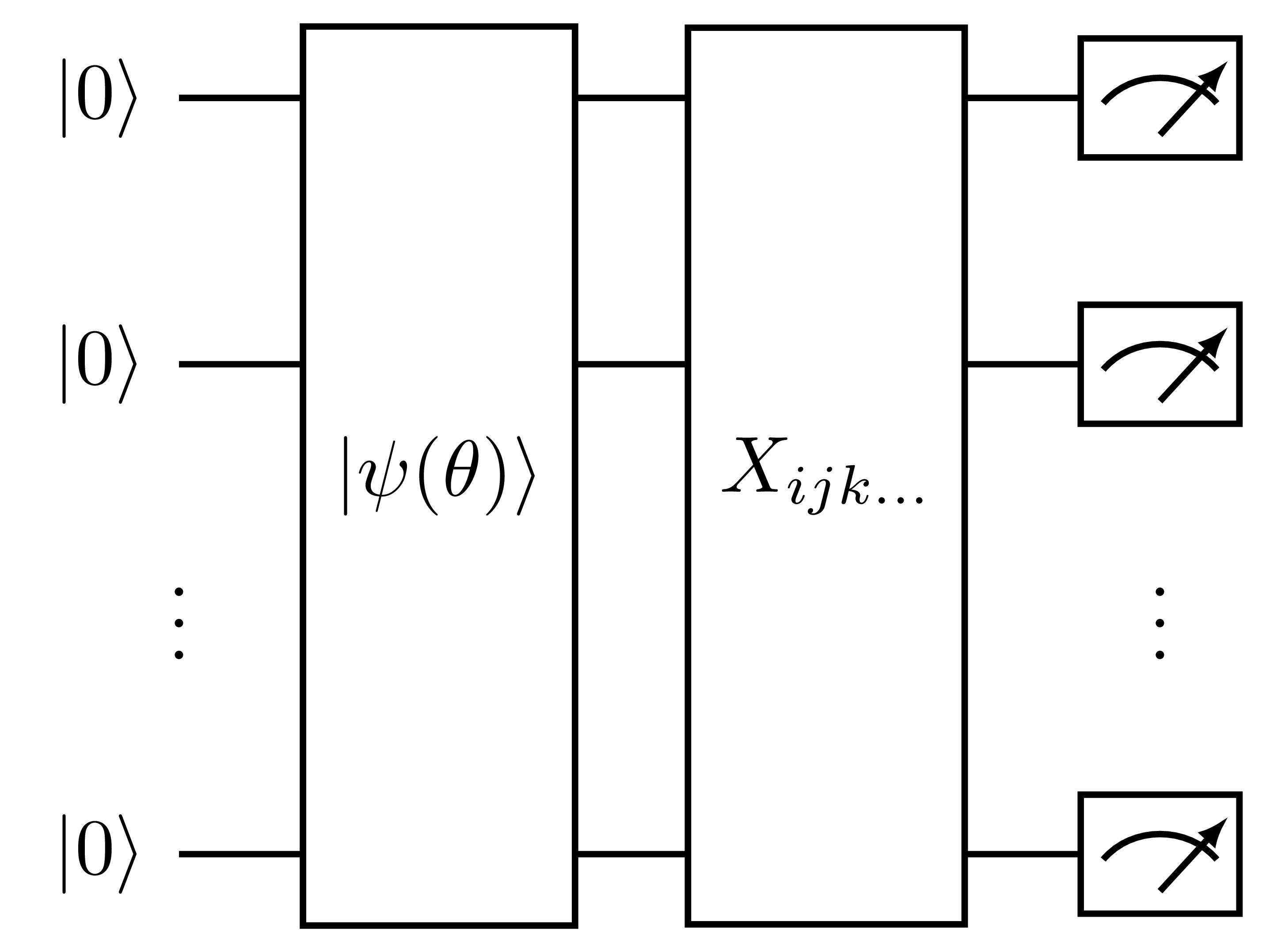
Fig. 8 Measurement circuit generated by PauliAveraging, where \(X_{ijk\dots}\) is the set of gates required to measure a commuting set of Pauli terms in the Hamiltonian.

Note

Rerunning a protocol will replace the results they contain. One can perform multiple evaluations with their results and then may choose to rerun to examine, for example, a different seed or number of shots.

HadamardTest

The HadamardTest protocol constructs one measurement circuit per Pauli word \(P_i\) in the operator. Each term is measured by performing a Hadamard test, which appends the Pauli string to the ansatz, controlled on an ancilla in the \(\ket{+}\) state.

We construct the measurement circuits similarly to above:

from inquanto.protocols import HadamardTest

protocol = HadamardTest(AerBackend(), shots_per_circuit=1000)
protocol.build_from({theta: -0.111}, energy)
protocol.run()

print("Number of circuits: ", protocol.n_circuit)

energy.evaluate(protocol.get_evaluator())

Number of circuits:  14

-1.140979169893277

One such measurement circuit for the Hamiltonian above is given by:

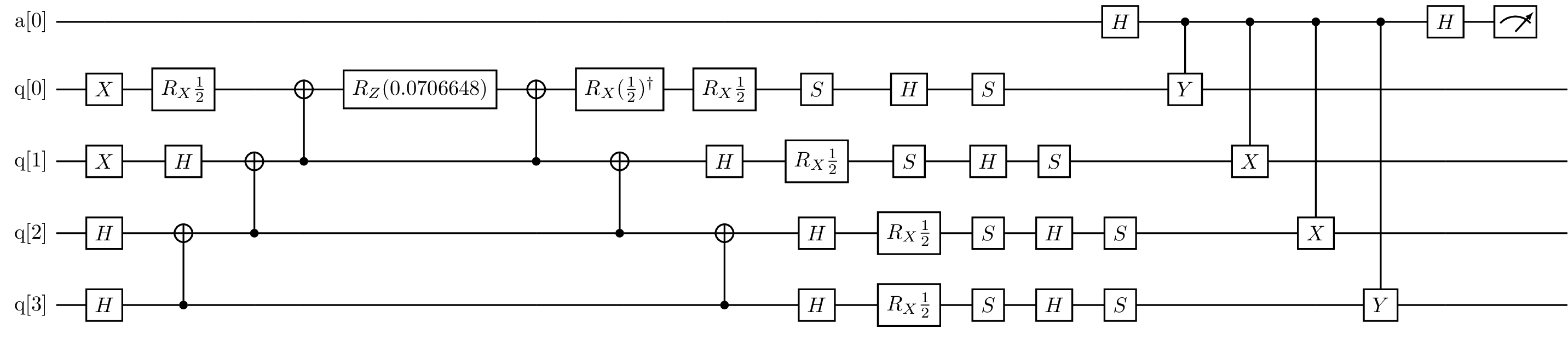
Fig. 9 Measurement circuit for the \(Y_0 X_1 X_2 Y_3\) term of the Hamiltonian, generated by the HadamardTest example above.

The expectation value of the corresponding Pauli string is determined by measuring the state of the ancilla qubit:

(41)\[\langle P_i \rangle = p(0) - p(1)\]

where \(p(b)\) is the probability of measuring the ancilla qubit in state \(b\in{0, 1}\). The expectation value of the full operator is then the sum over the product of weighted Pauli strings with the measured expectations.

In general, the measurement circuits generated by HadamardTest take the form:

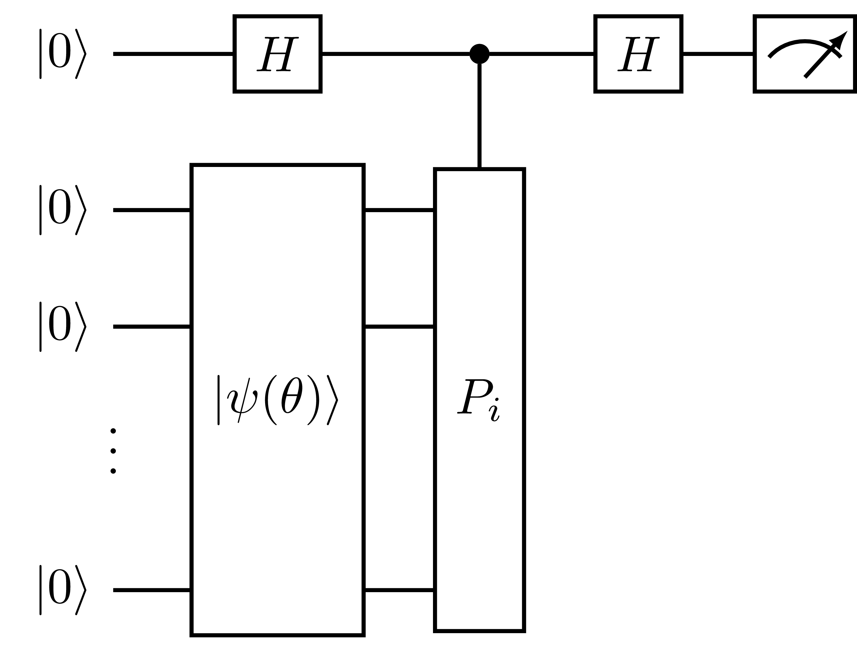
Fig. 10 Measurement circuit generated by HadamardTest.