AlgorithmVQS, AlgorithmMcLachlanRealTime and AlgorithmMcLachlanImagTime

These three classes implement variational quantum simulation (VQS) - a family of methods, solving the time-dependent Schrödinger equation (TDSE) by propagating a parameterized wavefunction (ansatz) using equations of motion (EOM), derived from one of the existing time-dependent variational principles (see [26] for a comprehensive review).

AlgorithmVQS is a general implementation, accepting any EOM in the form of a Computable expression parameter and any integrator. AlgorithmVQS assumes that EOM has a form of a linear ordinary differential equation (ODE), i.e. has the general form \(Ax = b\).

AlgorithmMcLachlanRealTime and AlgorithmMcLachlanImagTime are specialised classes. They implement the real and imaginary time evolution for a pure state respectively, following the EOM derived from the McLachlan variational principle, as provided in Eq. 12 of [26]. Following this reference, \(A\) is the real part of the ansatz metric tensor:

(30)\[A= \Re(\frac{\partial \langle\phi(\theta(t))|}{\partial \theta_i} \frac{\partial | \phi(\theta(t))\rangle}{\partial \theta_j})\]

and \(b\) is either:

(31)\[b = \Re(\frac{\partial \langle\phi(\theta(t))|}{\partial \theta_i} H | \phi(\theta(t))\rangle)\]

for imaginary-time evolution, or:

(32)\[b = \Im(\frac{\partial \langle\phi(\theta(t))|}{\partial \theta_i} H | \phi(\theta(t))\rangle)\]

for real-time evolution.

Below we provide an example of how these time evolution methods are applied, utilizing an ansatz to represent the wavepacket. The ansatz mixes the \(|1, 1, 0, 0>\) and \(|0, 0, 1, 1>\) states of a hydrogen molecule in the minimal basis set, allowing for an oscillation of the relative populations of those states during the time evolution.

First, we construct the H₂ Hamiltonian, as well as several observables that we would like to track during the wavepacket evolution (total energy, total particle number and orbital occupation number):

from inquanto.express import load_h5
from inquanto.spaces import FermionSpace

system = load_h5("h2_sto3g.h5", as_tuple=True)
hamiltonian_operator = system.hamiltonian_operator.qubit_encode()
fock_space = FermionSpace(4)
particle_number_operator = fock_space.construct_number_operator().qubit_encode()
orbital_number_operators = [
    op.qubit_encode() for op in fock_space.construct_orbital_number_operators()
]

Then, we define an ansatz that mixes the two configurations of interest. The configurations are one with both electrons in the first molecular spatial orbital (\(|1, 1, 0, 0 \rangle\), the Hartree-Fock ground state), and the other where both electrons are excited to the second spatial molecular orbital \((|0, 0, 1, 1 \rangle)\). Note that we add a global phase to the ansatz circuit and specify an initial condition for the wavepacket by setting the first ansatz parameter theta1 to \(\frac{\pi}{4}\):

from inquanto.ansatzes import TrotterAnsatz, CircuitAnsatz
from inquanto.operators import QubitOperatorList
from inquanto.core import OpType
from sympy import Symbol, pi

c1 = TrotterAnsatz(
    QubitOperatorList.from_string("theta1 [(1j, Y0 X1 X2 X3)]"), [1, 1, 0, 0]
).get_circuit()
c1.add_gate(OpType.from_name("U3"), [0, 0, Symbol("theta2") / pi], [0])  # Adds global phase
ansatz = CircuitAnsatz(c1)
initial = ansatz.state_symbols.construct_from_array([pi / 4, 0.0])

We are now in a position to initialize the integrator object. Here we use NaiveEulerIntegrator, but a more accurate SciPy integrator can be chosen as well - note the fine step size we need to obtain converged dynamics. Having created the integrator object, we construct the VQS algorithm object and then run the wavepacket propagation:

import numpy
from inquanto.minimizers import NaiveEulerIntegrator
from inquanto.algorithms import AlgorithmMcLachlanRealTime
from inquanto.protocols import SparseStatevectorProtocol
from pytket.extensions.qiskit import AerStateBackend

time = numpy.linspace(0, 5, 501)
integrator = NaiveEulerIntegrator(
    time, disp=False, linear_solver=NaiveEulerIntegrator.linear_solver_scipy_pinvh
)
protocol = SparseStatevectorProtocol(AerStateBackend())

algodeint = AlgorithmMcLachlanRealTime(
    integrator,
    hamiltonian_operator,
    ansatz,
    initial_parameters=initial,
)
solution = algodeint.build(
    protocol=protocol,
).run();

# TIMER BLOCK-0 BEGINS AT 2024-09-23 17:07:01.269914

# TIMER BLOCK-0 ENDS - DURATION (s): 35.9897364 [0:00:35.989736]

Finally, after the propagation has been completed, we can post-evaluate expectation values of the desired observables for each time step:

from inquanto.computables import ExpectationValue, ComputableList

evs_expression = ComputableList([
    ExpectationValue(ansatz, kernel) for kernel in [hamiltonian_operator, particle_number_operator, *orbital_number_operators]
])
runner = protocol.get_runner(evs_expression)

evs = algodeint.post_propagation_evaluation(runner)
evs = numpy.asarray(evs)

Here we plot the columns of the evs array to analyze results of the dynamics. We see that the electron number remains constant, while orbital occupations oscillate - this is due to the fact that we started by mixing the two electronic configurations, making the system non-stationary, and some electron (charge) dynamics is expected.

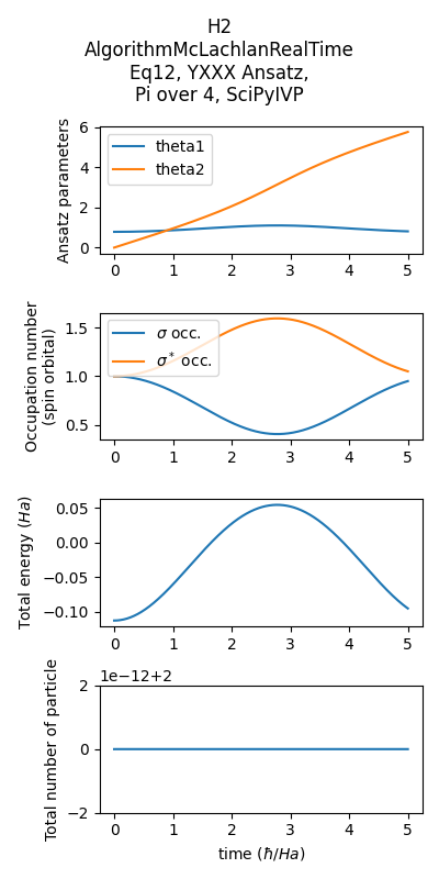
Fig. 6 Time evolution of various observables during a H₂ electronic wavepacket propagation.

However, total energy is not conserved, i.e. the propagation was not very accurate. The reason for this is that the EOM directly derived from McLachlan variational principle doesn’t properly account for the wavepacket phase evolution. This can be fixed by adding extra terms to it, as described in [26]. One can easily implement this EOM in InQuanto by creating a custom class, derived from the ComputableNode class and overriding the constructor and evaluate() method (see the time evolution examples). Then one can pass an instance of such class, together with the integrator of choice, to the AlgorithmVQS constructor, build and run it to perform a more accurate propagation.