Iterative Phase Estimation Algorithms

The iterative QPE algorithm, initially proposed by Kitaev [11, 18], runs a set of many QPE circuits with one ancilla qubit, each of which reads off partial information about the phase \(\phi\). The iterative QPE commonly uses the circuit as shown in Fig. 5.

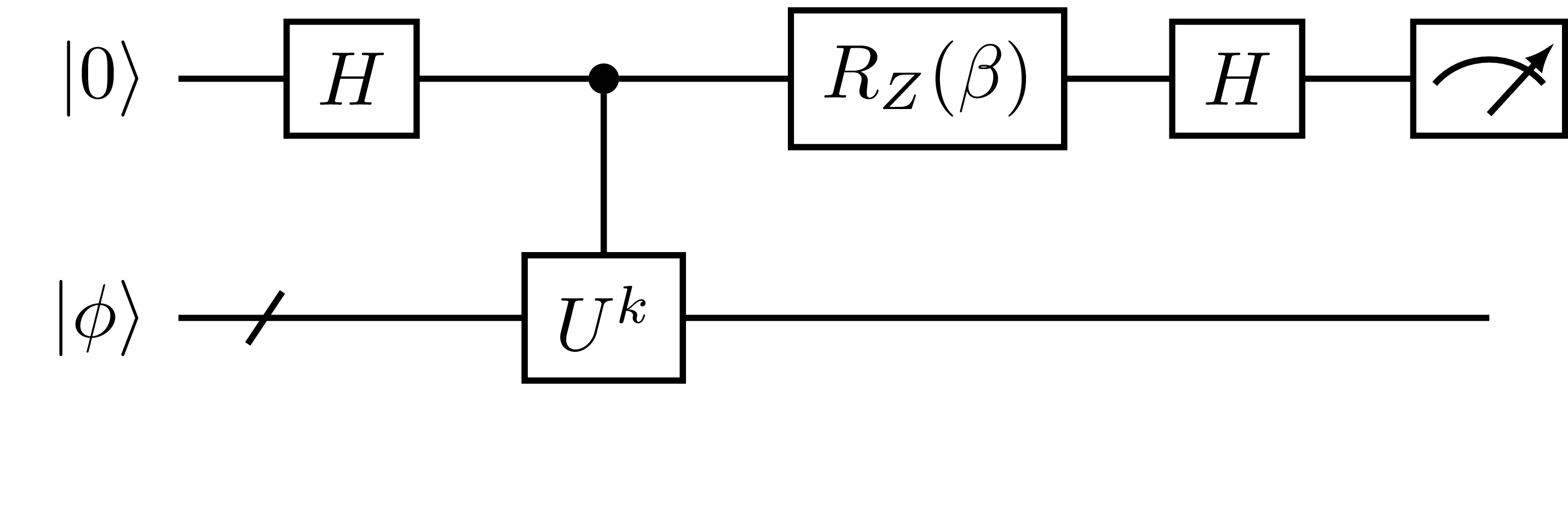
Fig. 5 Iterative QPE circuit parameterized by \(k \in \mathbb{N}\) and \(\beta \in [0, 2\pi)\).

The conditional probability of measuring \(m\) from this “basic measurement operation” [19] is expressed as

(27)\[p(m|\phi, k, \beta) = \frac{1 + \cos(k\phi + \beta - m\pi)}{2}\]

where \(m \in \{0, 1\}\). The basic idea of the iterative QPE algorithm is to perform the basic measurement operations on quantum hardware to generate samples and post-process them on classical hardware to infer the phase value. The iterative QPE algorithm needs a classical method for generating a sequence of circuit parameters \((k\), \(\beta)\), and that for post-processing the samples of \(m\).

As of now, InQuanto supports three iterative QPE algorithms:

• Kitaev’s QPE AlgorithmKitaevQPE [11]

• Information theory QPE AlgorithmInfoTheoryQPE [19]

• One flavor of Bayesian QPE AlgorithmBayesianQPE [20]

Kitaev’s QPE introduces the idea of replacing QFT with classical post-processing to produce a bit string of the phase value. Some algorithms [21, 22] inspired by Kitaev’s QPE become deterministic with no statistical inference under particular conditions. The information theory QPE [19] performs the maximum likelihood estimation. In this approach, one updates the distribution of the phase \(P(\phi)\) based on the “evidences” (i.e., measurement samples), similar to ideas in machine learning. Information theory QPE has inspired several stochastic QPE algorithms such as Bayesian QPE [23, 24, 25], including the one implemented in the InQuanto-Phayes extension [20]. We explain the primary usage of these algorithm classes in the following subsections.

To begin the demonstration, we load in a chemical system and trotterize the Hamiltonian to obtain qubit_operator_list. We also prepare an ansatz object state_prep as the initial state \(|\Phi\rangle\) using FermionSpaceAnsatzUCCSD. The time parameter defines the duration of the time evolution. These will be used to construct the controlled unitary operation \(\mathrm{ctrl-}U\).

from inquanto.express import get_system
from inquanto.mappings import QubitMappingJordanWigner
from inquanto.ansatzes import FermionSpaceAnsatzUCCSD

# Generate the spin Hamiltonian from the molecular Hamiltonian.
target_data = "h2_sto3g.h5"
fermion_hamiltonian, fermion_fock_space, fermion_state = get_system(target_data)
mapping = QubitMappingJordanWigner()
qubit_hamiltonian = mapping.operator_map(fermion_hamiltonian)

# Generate a list of qubit operators as exponents to be trotterized.
qubit_operator_list = qubit_hamiltonian.trotterize(trotter_number=1)

# The parameter `t` is physically recognized as the duration time in atomic units.
time = 0.25

# Preliminary calculated parameters.
ansatz_parameters = [-0.107, 0., 0.]

# Generate a non-symbolic ansatz.
ansatz = FermionSpaceAnsatzUCCSD(fermion_fock_space, fermion_state, mapping)
parameters = dict(zip(ansatz.state_symbols, ansatz_parameters))
state_prep = ansatz.subs(parameters)

Now we prepare the protocol that handles circuit-level operations.

from pytket.extensions.qiskit import AerBackend
from inquanto.protocols import IterativePhaseEstimation

# Prepare the pytket backend object.
backend = AerBackend()

# Construct the protocol to handle the iterative QPE circuits.
protocol = IterativePhaseEstimation(
    backend=backend,
    n_shots=30,
).build(
    state=state_prep,
    evolution_operator_exponents=qubit_operator_list * time,
)

This protocol object may be used in all the iterative QPE algorithms. Conceptually, IterativePhaseEstimation serves as a black box including quantum processors that takes \((k, \beta)\) of the circuit shown in Fig. 5 as input to return the measurement outcome \(m\).

Kitaev’s QPE

The basic idea of Kitaev’s QPE [11, 18] is to infer the phase bit by bit using the results of the basic measurement operations for \(k = 2^{n-1}, 2^{n-2}, \cdots, 2^{0}\), where \(n\) is the number of bits desired for representing the phase to the precision \(\epsilon\). \(\beta\) is chosen to be \(0\) and \(-\frac{\pi}{2}\) to estimate the real and imaginary part of \(e^{i2\pi\phi}\), respectively. This algorithm becomes similar to the Hadamard test if \(k\) is fixed to 1 and \(O(1/\epsilon^{2})\) measurement samples are considered. In Kitaev’s QPE, the circuit depth scales as \(O(1/\epsilon)\), whereas the number of shots scales \(O(\log \epsilon)\).

The inference procedure starts from the least significant bit. Suppose that the phase is represented with \(n+2\) bits, i.e., \(\phi = 0.\phi_{1}\phi_{2}\cdots\phi_{n}\phi_{n+1}\phi_{n+2}\). We estimate \(2^{n-1}\phi = 0.\phi_{n}\phi_{n+1}\phi_{n+2}\) similarly to the Hadamard test using the result of the basic measurement operation with \(k=2^{n-1}\). Then, \(\phi_{n-1}\) is determined so that \(0.\phi_{n-1}\phi_{n}\phi_{n+1}\) is closer to the phase estimate with \(k=2^{n-2}\). This inference process is repeated until we obtain the most significant bit \(\phi_{1}\).

In the cell below, we build the AlgorithmKitaevQPE object. The circuit depth is controlled by n_bits such that the maximum value of \(k\) is 2 ** (n_bits - 1).

from inquanto.algorithms import AlgorithmKitaevQPE

# Parameters for the Kitaev's QPE.
n_bits = 6

# Prepare the algorithm.
algorithm = AlgorithmKitaevQPE(
    n_bits=n_bits,
).build(
    protocol=protocol,
)

The build() method takes the IterativePhaseEstimation object. This may be replaced with any of the other iterative QPE protocols (see QPE protocols manual). Run the algorithm to evaluate the phase and thus the energy as

# Run the algorithm.
algorithm.run()

# Display the final results.
mu, precision = algorithm.final_value()
energy_mu = -mu / time
energy_resolution = precision / time
print(f"Energy     = {energy_mu:10.6f} hartree")
print(f"precision = {energy_resolution:10.6f} hartree")

Energy     =  -1.125000 hartree
precision =   0.015625 hartree

AlgorithmKitaevQPE returns the phase estimate and the precision to be used for computing the energy estimate. Note that the phase value is in the unit of half turns (i.e., \(\pi\)) following the pytket convention.

Information theory QPE

The basic idea of the information theory QPE is to estimate the phase \(\phi\) by maximizing the likelihood of the sequence of samples of the basic measurement operation [19]. Since the measurements are independent events, the likelihood of obtaining a sequence of \(s\) measurement outcomes \((m_{1}, m_{2}, \cdots, m_{s})\) for the sequence of parameters \(((k_{1},\beta_{1}),(k_{2},\beta_{2}), \cdots (k_{s},\beta_{s}))\) is expressed as

(28)\[ P( m_{1}, \cdots, m_{s} | \phi, k_{1}, \cdots, k_{s}, \beta_{1}, \cdots, \beta_{s} ) := \prod_{j}^{s} P(m_{j}|\phi, k_{j}, \beta_{j})\]

In practice, the phase \(\phi\) is discretized as \(\phi_{l}=\frac{l}{M}\), where \(l = 0, 1, \cdots, M-1\), and perform \(s\) basic measurement operations for randomly selected \(k \in [1, k_{\mathrm{max}})\) and \(\beta \in [0, 2\pi)\) from uniform distribution, where \(k_{\mathrm{max}}\) is the maximum value of \(k\) and \(M\) is the number of grid points to resolve \(\phi\) Then, the probability distribution is calculated with Eq. (28) to estimate the phase value. In the initial proposal in [19], the phase value is obtained as

(29)\[\phi = \underset{l} {\operatorname{argmax}} P( m_{1}, \cdots, m_{s} | \phi_{l}; k_{1}, \cdots, k_{s}, \beta_{1}, \cdots, \beta_{s} )\]

In InQuanto, it is generalized to return the mean \(\mu\) and the standard deviation \(\sigma\) of \(P( m_{1}, \cdots, m_{s} | \phi_{l}; k_{1}, \cdots, k_{s}, \beta_{1}, \cdots, \beta_{s})\).

Now we demonstrate AlgorithmInfoTheoryQPE. We prepare the protocol object similarly to the Kitaev’s QPE case but with n_shots=1 to perform the one-shot experiment for each pair of the circuit parameters.

# Construct the protocol to handle the iterative QPE circuits.
protocol = IterativePhaseEstimation(
    backend=backend,
    n_shots=1,
).build(
    state=state_prep,
    evolution_operator_exponents=qubit_operator_list * time,
)

Then we construct the AlgorithmInfoTheoryQPE with some parameters specifying the computational condition of the information theory QPE.

from inquanto.algorithms import AlgorithmInfoTheoryQPE

# Parameters.
n_bits = 6
resolution = 2 ** (n_bits + 4)
k_max = 2 ** (n_bits - 1)
n_samples = 50

# Set up the algorithm object.
algorithm = AlgorithmInfoTheoryQPE(
    resolution=resolution,
    k_max=k_max,
    n_samples=n_samples,
).build(
    protocol=protocol,
)

Run the algorithm to produce the energy estimate similarly to the case of Kitaev’s QPE.

# Run the algorithm.
algorithm.run()

# Display the final results.
mu, sigma = algorithm.final_value()
energy_mu = -mu / time
energy_sigma = sigma / time
print(f"Energy(mu)    = {energy_mu:10.6f} hartree")
print(f"Energy(sigma) = {energy_sigma:10.6f} hartree")

Energy(mu)    =  -1.137860 hartree
Energy(sigma) =   0.010397 hartree