Protocols for Phase Estimation

Quantum phase estimation (QPE) [11, 12, 13, 14] is a quantum algorithm used to estimate the phase \(\phi \in [0, 1)\) of a given unitary operator \(U\) and eigenstate \(|\phi\rangle\) satisfying

(62)\[U|\phi\rangle = e^{i2\pi\phi} |\phi\rangle .\]

There are two main approaches to QPE algorithms, i.e., QPE based on the quantum Fourier transform (QFT) and QPE based on classical post-processing. The former is referred to as canonical QPE. It requires as many ancilla qubits as is necessary for representing the phase to the desired precision. The latter is called iterative QPE. The phase value is inferred by analyzing the samples obtained with the basic measurement operation with one ancilla qubit. Currently, InQuanto supports the protocol layer for the iterative QPE algorithms.

IterativePhaseEstimation

Iterative QPE algorithms commonly use the circuit below.

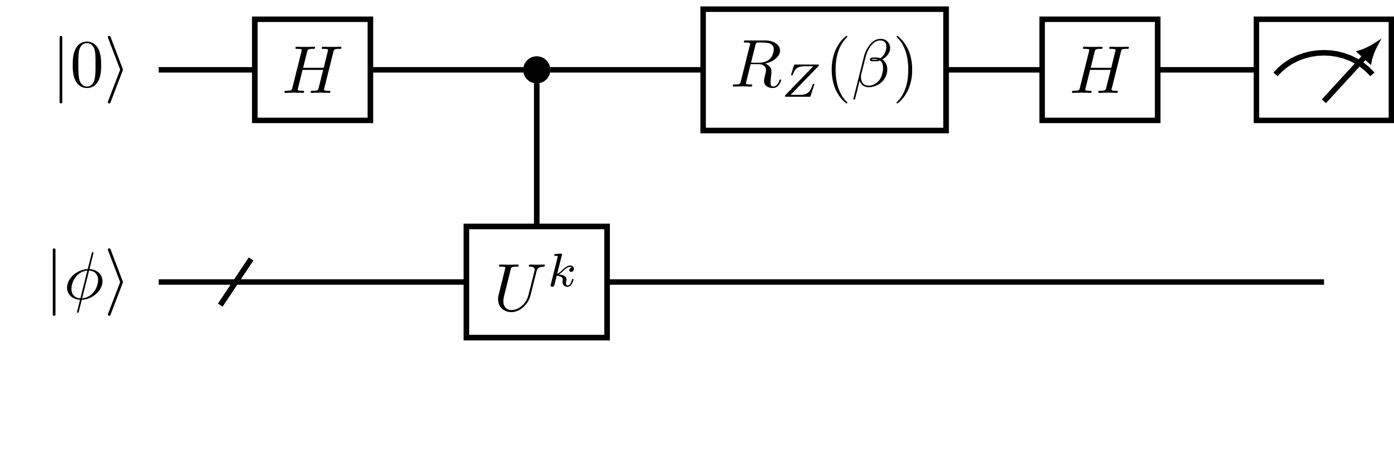
Fig. 23 Iterative QPE circuit parameterized by \(k \in \mathbb{N}\) and \(\beta \in [0, 2\pi)\).

Conceptually, IterativePhaseEstimation serves as a black box taking \((k, \beta)\) as input to return the measurement sample(s) \(m \in \{0, 1\}\) as output. The probability of measuring \(m\) from this circuit is expressed as

(63)\[P(m|\phi, k, \beta) = \frac{1 + \cos(k\phi + \beta - m\pi)}{2}\]

The iterative QPE protocols return samples of \(m\) to be post-processed by the higher-level routine, such as the objects of the algorithm layer of InQuanto.

To demonstrate the primary usage of iterative QPE protocols, consider the example below with the following setup for example:

(64)\[\begin{split}U = U_{1}(\alpha) = \left(\begin{array}{cc} 1 & 0 \\ 0 & e^{i2\pi\alpha} \end{array}\right)\end{split}\]

and the initial state is

(65)\[|\phi\rangle = |1\rangle\]

In this case, the phase readout will be \(2\pi k \alpha\). Consider the case of \(\beta = -2\pi k\alpha\) to always obtain measurement outcome \(m = 0\) for convenience.

To begin, we must build some objects required for the iterative QPE protocol.

from pytket.circuit import Circuit, OpType
from pytket.extensions.qiskit import AerBackend
from inquanto.protocols import IterativePhaseEstimation

# Eigenphase for example.
alpha = 1.0 / 8

# Protocol parameter.
n_shots = 10

# Prepare a function to return the ctrl-U circuit.
def get_ctrlu(k: int) -> Circuit:
    ctrlu = Circuit(2)
    ctrlu.add_gate(OpType.CU1, 2 * k * alpha, [0, 1])
    return ctrlu

# Prepare the circuit for the state preparation.
init_state = Circuit(1).X(0)

# pytket Backend.
backend = AerBackend()

Then we construct and build the IterativePhaseEstimation object.

# Initialize and build the protocol, and then set the circuit parameter.
protocol = IterativePhaseEstimation(
    backend=backend,
    n_shots=n_shots,
).build_from_circuit(
    get_ctrlu=get_ctrlu,
    state=init_state,
);

# Set the circuit parameter.
k = 4
beta = -2 * k * alpha   # To ensure the measurement outcome is always 0.
protocol.update_k_and_beta(k, beta)

# Run the protocol to get the measurement outcome
protocol.run()
protocol.get_measurement_outcome()

[0, 0, 0, 0, 0, 0, 0, 0, 0, 0]

To make it more like a chemistry problem, one can pass the QubitOperatorList as the exponents to be trotterized as \(U = e^{-iHt}\).

from inquanto.operators import QubitOperator
from inquanto.ansatzes import CircuitAnsatz

# Input for generating the CTRL-U gate.
time = 1.0
hamiltonian = QubitOperator("Z0", 0.5)
qopl = hamiltonian.trotterize()

# Ansatz circuit for the state preparation.
prep_ansatz = CircuitAnsatz(Circuit(1))

# Construct and build the protocol, then update the circuit parameter.
protocol = IterativePhaseEstimation(
    backend=backend,
    n_shots=n_shots,
).build(
    state=prep_ansatz,
    evolution_operator_exponents=qopl * time,
)

# Set the circuit parameters.
k = 10
beta = 0.56789
protocol.update_k_and_beta(k, beta)

# Run the protocol.
protocol.run()

# Get the measurement outcome.
protocol.get_measurement_outcome()

[1, 0, 0, 1, 0, 0, 0, 0, 0, 1]

The measurement outcome may be a random sequence of 0 and 1, the probability of which is determined by (63).

This protocol may be helpful as a subroutine of iterative QPE algorithms. The higher-level workflow should manage the classical pre- and post-processing methods. The pre-processing here means the generation of the samples of \((k, \beta)\), whereas post-processing implies the interpretation of measurement outcome \(m\) on classical computers, which could be the evaluation of the expectation value \(\langle e^{-iHt} \rangle\), the inference procedure using the likelihood (63), and so on, depending on the iterative QPE algorithm. Once the protocol object is built, update_k_and_beta(), run(), and get_measurement_outcome() are used by those higher-level algorithms without concerning the inside of the protocol object. See Iterative QPE algorithms section for more about the application.

IterativePhaseEstimationQuantinuum

IterativePhaseEstimation is designed for a noiseless backend to be free from backend-specific options. However, such options are essential for experiments on a noisy backend such as real quantum hardware. IterativePhaseEstimationQuantinuum is designed for a noisy simulation to get the most out of the pytket Quantinuum backend.

One of the remarkable features provided by this class is the logical qubit encoding using an error detection code [35]. Users can perform logical qubit experiments of iterative QPE algorithms, thanks to the features of Quantinuum H-Series hardware, including high-fidelity operations for all-to-all connected qubits, mid-circuit measurement, qubit reuse, and conditional logic.

Currently, the \([[n+2, n, 2]]\) error detection code (dubbed iceberg code) proposed by C. Self, M. Benedetti, D. Amaro [35] is available. The experimental demonstration of the iterative QPE for a hydrogen molecule with the iceberg code has been performed by K. Yamamoto, S. Duffield, Y. Kikuchi, and David Muñoz Ramo [20].

First let us prepare the objects to build IterativePhaseEstimationQuantinuum

from pytket.circuit.display import render_circuit_jupyter
from pytket.extensions.quantinuum import QuantinuumBackend
from inquanto.operators import QubitOperator

# pytket Backend.
# backend = QuantinuumBackend(device_name="H1-1E")
backend = AerBackend()

hamiltonian = QubitOperator("Z0", 0.25) + QubitOperator("X0", -0.33)
qopl = hamiltonian.trotterize()

# Ansatz circuit for the state preparation.
prep_ansatz = CircuitAnsatz(Circuit(1))

# Circuit parameters.
k = 4
beta = 0.25

This simple example of IterativePhaseEstimationQuantinuum is almost compatible with IterativePhaseEstimation as

from inquanto.protocols import (
    IterativePhaseEstimationQuantinuum,
    CompilationLevelQuantinuum,
    CircuitEncoderQuantinuum,
)
# Construct and build the protocol, then update the circuit parameter.
protocol = IterativePhaseEstimationQuantinuum(
    backend=backend,
    n_shots=n_shots,
    compilation_level=CompilationLevelQuantinuum.ENCODED,
).build(
    state=prep_ansatz,
    evolution_operator_exponents=qopl,
    encoding_method=CircuitEncoderQuantinuum.PLAIN,
).update_k_and_beta(k, beta)

# Display the encoded circuit.
circ = protocol.get_circuits()[0]
render_circuit_jupyter(circ)

Note that we can control the backend-specific compilation by specifying compilation_level. One can activate the logical qubit encoding with the encoding_method option as

from inquanto.protocols import IcebergOptions

# Construct and build the protocol, then update the circuit parameter.
protocol = IterativePhaseEstimationQuantinuum(
    backend=backend,
    n_shots=n_shots,
    compilation_level=CompilationLevelQuantinuum.ENCODED,
).build(
    state=prep_ansatz,
    evolution_operator_exponents=qopl,
    encoding_method=CircuitEncoderQuantinuum.ICEBERG,
    encoding_options=IcebergOptions(
        syndrome_interval=2,
        sx_insertion=True,
    )
).update_k_and_beta(k, beta)

# Display the encoded circuit.
circ = protocol.get_circuits()[0]
render_circuit_jupyter(circ)

The encoding_method may be accompanied by encoding_options to set the encoding-method-specific options. In this case, we set the syndrome_interval=2 to perform the syndrome measurement (error detection) [35], and sx_insertion=True to enable the simple dynamical decoupling for the error suppression [20]. Although the circuits look very different from each other, the key methods such as update_k_and_beta() and get_measurement_outcome() work essentially in the same manner, i.e., the encoding of circuits and the decoding of measurement outcomes are performed within the protocol layer.

Circuit optimization strategy may differ from the unencoded physical qubit implementation if we use the logical qubit encoding. To help the circuit optimization, IterativePhaseEstimationQuantinuum has additional options, such as terms_map and paulis_map.

The terms_map option of the build() method is used for replacing a Pauli string of \(H\) with another Pauli string. Typically, we use it to introduce a “dummy” qubit [20] to enable the logical qubit encoding by the iceberg code, as the iceberg code requires a code block consisting of even number qubits. Let us consider the following qubit Hamiltonian, for example.

(66)\[H = gX_{0}X_{1},\]

where \(g \in \mathbb{R}\) is a coefficient. We can easily convert it into \(H = gI_{0}X_{1}X_{2}\) without reconstructing the Hamiltonian by using terms_map option as

from pytket.circuit import Qubit
from pytket.pauli import Pauli, QubitPauliString
from inquanto.operators import QubitOperator

# Prepare a Hamiltonian.
qpol = QubitOperator("X0 X1", 0.25).trotterize()

# Prepare the terms_map object.
qps_xx = QubitPauliString([Qubit(0), Qubit(1)], [Pauli.X, Pauli.X])
qps_ixx = QubitPauliString([Qubit(1), Qubit(2)], [Pauli.X, Pauli.X])
terms_map = {qps_xx: qps_ixx}

# Prepare the state.
init_state = CircuitAnsatz(Circuit(3))

Then, construct the protocol to generate the encoded circuit as

# Initialize and build the protocol.
protocol = IterativePhaseEstimationQuantinuum(
    backend=None,
    compilation_level=CompilationLevelQuantinuum.ENCODED,
).build(
    state=init_state,
    evolution_operator_exponents=qpol,
    encoding_method=CircuitEncoderQuantinuum.ICEBERG,
    terms_map=terms_map,
).update_k_and_beta(k=1, beta=0.0)

# Display the circuit.
circ = protocol.get_circuits()[0]
render_circuit_jupyter(circ)

The dummy qubit undergoes no logical operations in general, but we may use it for circuit optimization. For example, the \(X\) operator acting on this dummy qubit serves as a stabilizer if the dummy qubit is initialized as \(|+\rangle\). We can use this additional stabilizer for the circuit optimization to obtain a Pauli string to optimize the circuit by exploiting the other stabilizers.

# Set the Puali map object.
qubits = [Qubit(i) for i in range(4)]
qps_zixx = QubitPauliString(qubits, [Pauli.Z, Pauli.I, Pauli.X, Pauli.X])
qps_zxxx = QubitPauliString(qubits, [Pauli.Z, Pauli.X, Pauli.X, Pauli.X])
paulis_map = {qps_zixx: qps_zxxx}

# Initialize and build the protocol, and then set the circuit parameter.
protocol = IterativePhaseEstimationQuantinuum(
    backend=None,
    compilation_level=CompilationLevelQuantinuum.ENCODED,
).build(
    state=init_state,
    evolution_operator_exponents=qpol,
    encoding_method=CircuitEncoderQuantinuum.ICEBERG,
    encoding_options=IcebergOptions(
        n_plus_states=2,
    ),
    terms_map=terms_map,
    paulis_map=paulis_map,
).update_k_and_beta(k=1, beta=0.0)

# Display the circuit.
circ = protocol.get_circuits()[0]
render_circuit_jupyter(circ)

See [20] for technical details.

IterativePhaseEstimationStatevector

Some forms of iterative QPE (such as Kitaev’s QPE) use the probability distribution of measurement outcome \(m\), rather than the sequence of \(m\). Exact probability distribution will be useful for quick and reliable prototyping. IterativePhaseEstimationStatevector has such a feature, get_distribution().

from inquanto.protocols import IterativePhaseEstimationStatevector

# Eigenphase in the pytket convention (angle is in the unit of half turn).
phase = 1.0 / 8

# Protocol arameters.
k = 4
beta = -2 * k * phase   # To make sure the measurement outcome is always 0.
n_shots = 10

# Prepare a function to return the ctrl-U circuit.
def get_ctrlu(k: int) -> Circuit:
    ctrlu = Circuit(2)
    ctrlu.add_gate(OpType.CU1, 2 * k * phase, [0, 1])
    return ctrlu

# Prepare the circuit for the state preparation.
init_state = Circuit(1).X(0)

# pytket Backend.
backend = AerBackend()

# Initialize and build the protocol, and then set the circuit parameter.
protocol = IterativePhaseEstimationStatevector(
).build_from_circuit(
    get_ctrlu=get_ctrlu,
    state=init_state,
).update_k_and_beta(k, beta)

protocol.run()
protocol.get_distribution()

{(0,): 1.0, (1,): 0.0}

Internally, this class classically diagonalizes the unitary to obtain the eigenvalues and calculate the eigenstate population of the initial state to weight the likelihood functions. Note that this exact diagonalization may take a long time, even for a modest system size.