NEVPT2 and AC0 energy corrections
In this tutorial, we will explore the use of NEVPT2 (N-electron valence state perturbation theory with second-order approximations) as a perturbation theory approach that can be used to improve the accuracy of our electronic structure calculations beyond the mean-field methods like Hartree-Fock or density functional theory (DFT) when running quantum computations. Our focus will be on the Li\(_2\) system, which presents a higher level of complexity compared to the H\(_2\) molecule while still maintaining a reasonable level of simplicity.
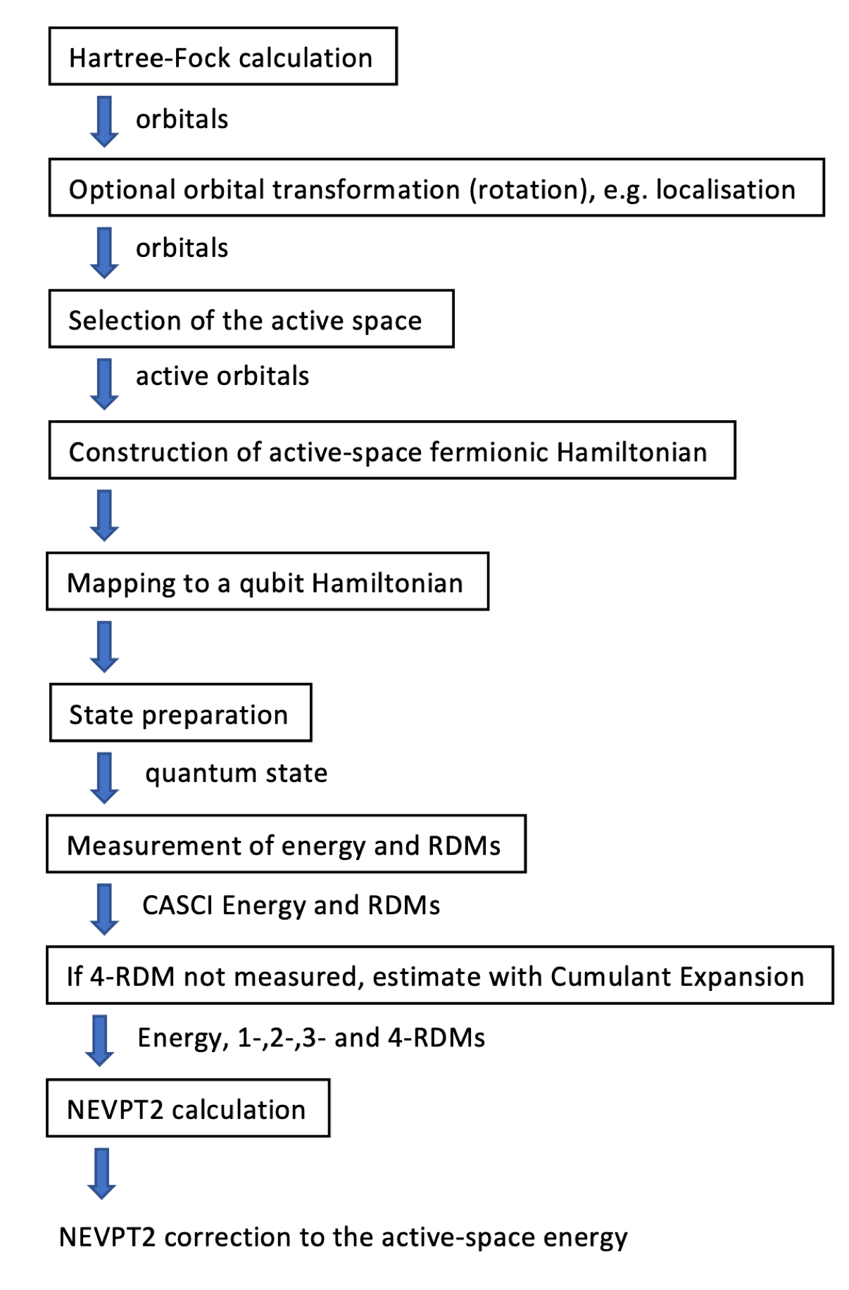
A novel approach that combines quantum and classical methods for strongly contracted N-electron Valence State 2nd-order Perturbation Theory (SC-NEVPT2) is implemented in InQuanto. In this method, the static correlation effects typically handled by the Complete Active Space Configuration Interaction (CASCI) step are replaced by quantum computer simulations. Specifically, we use a quantum computer to measure n-particle Reduced Density Matrices (n-RDMs), and these measurements are then employed in a classical SC-NEVPT2 calculation to approximate the remaining dynamic electron correlation effects. Additionally, we explore the application of the cumulant expansion to either approximate the entire 4-RDM matrix or only its zero elements. This work not only showcases noiseless state-vector quantum simulations but also marks the first instance of a hybrid quantum-classical calculation for multi-reference perturbation theory, with the quantum component executed on a quantum computer.
The flowchart depicted below provides a concise overview of this approach, with the “State preparation” step in the current implementation being handled by the Variational Quantum Eigensolver (VQE). For further details and comprehensive information about this approach, see Krompiec & Muñoz Ramo (2022).
As an alternative approach, we can calculate the energy’s AC0 correction using the provided density matrices. Here, one- and two-particle reduced density matrices are employed to account for electron correlation effects. The AC-CAS (Adiabatic Connection Construction and Extended Random Phase Approximation for Complete Active Space Wave Functions) is a computational method within the field of quantum chemistry employed to investigate the electronic structure and properties of molecular systems. This method combines two crucial techniques: the adiabatic connection (AC) method and the complete active space (CAS) approach, along with the extended random phase approximation.
In this context, we have utilized the AC0-CAS method, known as the First-Order Expansion of the AC Integrand at α = 0. Starting with α = 0 essentially means beginning with the simplest form of the system, which corresponds to the reference system with non-interacting electrons. Subsequently, electron-electron interactions are introduced perturbatively, taking into account only the first-order effects. This approach is commonly employed in quantum chemistry to make calculations more manageable while still capturing some degree of electron correlation. AC0-CAS proves particularly valuable in striking a balance between computational efficiency and accuracy in electronic structure calculations. While it may not encompass the full spectrum of electron correlation effects, it can still yield reasonably accurate results for a broad range of molecular systems. Further information on the AC0 correction can be found in Pastorczak & Pernal (2018).
The following steps outline the process:
Define the system
Compute the NEVPT2 correction to the energy using RDMs from VQE
Compute the NEVPT2 correction to the energy using RDMs from CASCI
Compute the AC0 correction to the energy
The first step is to run Hartree-Fock (HF) calculations and in our case restricted Hartree-Fock (RHF) with the 6-31G basis set. We use an InQuanto-PySCF driver to perform the molecular RHF calculations, and store the resulting Hamiltonian after it is qubit encoded.
Parameters used:
geometry – Molecular geometry.
basis – Atomic basis set valid for Mole class.
charge – Total charge.
transf – Orbital transformer.
frozen – Frozen orbital information.
point_group_symmetry – Enable point group symmetry.
verbose – Control PySCF verbosity.
The FromActiveSpace function aids in determining the frozen orbital list based on the information provided about the active space. In this context, ncas represents the number of active orbitals, and nelecas represents the number of active electrons. In this case, we have opted to perform postprocessing of orbitals using the Complete Active Space Self-Consistent Field (CASSCF) method to construct molecular integrals. We pass two key parameters, ncas (the number of active spatial
orbitals) and nelecas (the number of active electrons), to pyscf.mcscf.CASSCF. This approach allows us to effectively utilize the CASSCF method for the subsequent steps involving molecular integrals.
[ ]:
import warnings
warnings.filterwarnings('ignore')

from inquanto.extensions.pyscf import ChemistryDriverPySCFMolecularRHF, CASSCF, FromActiveSpace

geometry = [["Li", [0.0, 0.0, 0.0]], ["Li", [2.63, 0.0, 0.0]]]

ncas, nelecas = 4, 2
driver = ChemistryDriverPySCFMolecularRHF(
    basis="6-31G",
    charge=0,
    geometry=geometry,
    transf=CASSCF(ncas, nelecas),
    frozen=FromActiveSpace(ncas, nelecas),
    point_group_symmetry=True,
    verbose=0,
)

driver.run_hf()
-14.864996327400355
The get_system function is responsible for computing the fermionic Hamiltonian operator, Fock space, and Hartree Fock state. The qubit_encode function carries out qubit encoding, utilizing the mapping class associated with the current integral operator. The default mapping is Jordan-Wigner (used throughout this tutorial).
[ ]:
chemistry_hamiltonian, space, state = driver.get_system()
qubit_hamiltonian = chemistry_hamiltonian.qubit_encode()
To construct our ansatz for the specified fermion space and fermion state, we have employed the Chemically Aware Unitary Coupled Cluster with singles and doubles excitations (UCCSD).
[ ]:
from inquanto.ansatzes import FermionSpaceAnsatzChemicallyAwareUCCSD

ansatz = FermionSpaceAnsatzChemicallyAwareUCCSD(space, state)
Here, we conduct a simple VQE experiment to determine the ground state energy of our system. For a more comprehensive guide on performing VQE calculations using InQuanto on quantum computers, we recommend referring to the VQE tutorial. To define where the computation is performed we set the backend to AerStateBackend().
[ ]:
from pytket.extensions.qiskit import AerStateBackend
from inquanto.express import run_vqe
from inquanto.minimizers import MinimizerRotosolve

backend = AerStateBackend()

vqe = run_vqe(
    ansatz,
    qubit_hamiltonian,
    backend=backend,
    with_gradient=False,
    minimizer=MinimizerRotosolve(),
)
# TIMER BLOCK-1 BEGINS AT 2024-02-15 19:05:04.004600
# TIMER BLOCK-1 ENDS - DURATION (s):  0.6568890 [0:00:00.656889]
The InQuanto inquanto.spaces.QubitSpace.symmetry_operators_z2 function is employed to retrieve a list of symmetry operators applicable to our system. These symmetry operators are associated with the point group, spin parity, and particle number parity \(\mathbb{Z}_2\) symmetries that uphold a specific symmetry sector.
[ ]:
from inquanto.spaces import QubitSpace

symmetry_operators = QubitSpace(space.n_spin_orb).symmetry_operators_z2(
    qubit_hamiltonian
)
The NEVPT2 implementation in PySCF, which is used in InQuanto, utilizes Pre-Density Matrices (PDMs). These PDMs are defined using the same creation and annihilation operators as the corresponding Reduced Density Matrices (RDMs), but they are applied in a different order. The class inquanto.computables.composite.PDM1234RealComputable computes the 1st, 2nd, 3rd, and 4th PDMs for a specific state, as determined by the provided ansatz and parameters.
Parameters used:
space – Fermion occupation space spanned by this RDM.
ansatz – Ansatz state with respect to which expectation values are computed.
encoding – Fermion to qubit mapping.
symmetry_operators – \(\mathbb{Z}_2\) symmetries of the Hamiltonian.
cas_elec – Number of active electrons.
cas_orbs – Number of active orbitals.
The computation of the 4-RDM can be computationally expensive. Therefore, for chemical systems with more than 3 active electrons (where the 4-RDM is non-negligible), we estimate the 4-PDM using the cumulant expansion approximation. This approximation is set by the class parameter cu4, which is True by default. If this parameter is set to False, the 4-PDM is directly computed. For further insights into the impact of this approximation on both computational cost and accuracy, please
refer to Krompiec & Muñoz Ramo (2022).
[ ]:
from inquanto.computables.composite import PDM1234RealComputable
from inquanto.mappings import QubitMappingJordanWigner

pdm_computables = PDM1234RealComputable(
    space=space,
    ansatz=ansatz,
    encoding=QubitMappingJordanWigner(),
    symmetry_operators=symmetry_operators,
    cas_elec=nelecas,
    cas_orbs=ncas,
)
Subsequently, the evaluation PDMs is carried out using the inquanto.protocols.SparseStatevectorProtocol class, which is designed for sparse statevector calculations while utilizing caching. The get_evaluator method is employed to generate and provide a function (evaluator) that receives a specific quantum computable and computes it based on its type.
[ ]:
from inquanto.protocols import SparseStatevectorProtocol

pdms = pdm_computables.evaluate(
    SparseStatevectorProtocol(backend).get_evaluator(vqe.final_parameters)
)
Finally, the get_nevpt2_correction function is employed to calculate the strongly contracted NEVPT2 correction to the energy using the provided density matrices.
[ ]:
nevpt2_energy = driver.get_nevpt2_correction(pdms)
In a similar way, using the same driver, we can calculate the AC0 energy correction, but this time we will make use of the inquanto.computables.composite.SpinlessNBodyRDMArrayRealComputable class which calculates a general n-body RDM \(\Gamma_{n...m}^{i...j} = \left \langle \Psi_0 \left | \hat{E}_{n...m}^{i...j} \right |\Psi_0 \right \rangle\) where \(\hat{E}_{n...m}^{i...j}\) is a spin-traced excitation operator. For example, in the one-body case this is:
And in the two-body case:
Spin-traced 1-RDM and 2-RDM refer to reduced density matrices where the electron spin degrees of freedom have been summed over or “traced out.” This is done to obtain the spatial (orbital) electronic density matrices, which describe the distribution of electrons in terms of their spatial coordinates or orbitals, while ignoring their spin states.
Parameters used:
n – Rank of the spin-traced RDM (n-RDM).
fermion_space – Fermion space where the operators are defined.
ansatz – Ansatz with respect to which the expectation values are computed.
encoding – Qubit encoding from fermion space to qubit space.
symmetry_operators – List of \(\mathbb{Z}_2\) symmetries of the Hamiltonian.
taperer – Optional taperer object.
The inquanto.protocols.SparseStatevectorProtocol class and its get_evaluator method are utilized in the same way as previously.
[ ]:
from inquanto.computables.composite import SpinlessNBodyRDMArrayRealComputable
from inquanto.computables import ComputableList

rdm_computable = ComputableList(
    [
        SpinlessNBodyRDMArrayRealComputable(
            n=n,
            fermion_space=space,
            ansatz=ansatz,
            encoding=QubitMappingJordanWigner(),
            symmetry_operators=symmetry_operators,
            taperer=None,
        )
        for n in (1, 2)
    ]
)
rdm_computed = rdm_computable.evaluate(
    SparseStatevectorProtocol(backend).get_evaluator(vqe.final_parameters)
)

dm1 = rdm_computed[0]
dm2 = rdm_computed[1]
The get_ac0_correction function is employed to compute the AC0 correction to the energy from the provided density matrices.
[ ]:
ac0_energy = driver.get_ac0_correction((dm1, dm2))
We can now compare the various energy results.
An alternative approach would be to perform CASSCF calculations to obtain the PDMs and RDMs. In this process, we initially compute the PDMs by executing the CASSCF calculation using the PySCF package. For additional details, you can refer to the relevant PySCF documentation. Following this, our RHF InQuanto driver has been created and the HF orbital coefficients have been replaced with those obtained from the CASSCF calculation in order to improve the description of the orbitals and enhance the representation of the system.
[ ]:
from pyscf import gto, scf, fci, mcscf

mf = gto.M(atom=geometry, basis="6-31g").apply(scf.RHF).run()
mc = mcscf.CASSCF(mf, ncas, nelecas )
mc.run()
mf.mo_coeff=mc.mo_coeff
(pdm1, pdm2, pdm3, pdm4) = fci.rdm.make_dm1234(
    "FCI4pdm_kern_sf", mc.ci, mc.ci, ncas, nelecas
)

driver_casscf = ChemistryDriverPySCFMolecularRHF.from_mf(
    mf, frozen=FromActiveSpace(ncas, nelecas)(mf)
)
converged SCF energy = -14.8652654987828
CASSCF energy = -14.8887816132799
CASCI E = -14.8887816132799  E(CI) = -0.619242398867161  S^2 = 0.0000000
We can once again employ the get_nevpt2_correction function to compute the strongly contracted NEVPT2 correction to the energy.
[ ]:
nevpt2_energy_casscf = driver_casscf.get_nevpt2_correction(rdms=(pdm1, pdm2, pdm3, pdm4))
Sr    (-1)',   E = 0.00000000000063
Si    (+1)',   E = -0.00001592230223
Sijrs (0)  ,   E = -0.00022778404137
Sijr  (+1) ,   E = -0.00007024183793
Srsi  (-1) ,   E = -0.00023752538838
Srs   (-2) ,   E = -0.00127421582345
Sij   (+2) ,   E = -0.00002668012481
Sir   (0)' ,   E = -0.00013325632488
Nevpt2 Energy = -0.001985625842400
The make_dm1234 function in PySCF calculates the PDMs, which do not directly correspond to the 1-, 2-, 3-, and 4-particle density matrices. The reorder_dm12 function is then used to convert these PDMs into the actual 1- and 2-particle density matrices.
[ ]:
rdm1, rdm2 = fci.rdm.reorder_dm12(pdm1, pdm2)

ac0_energy_casscf = driver_casscf.get_ac0_correction((rdm1, rdm2))
As the final step, we can compare the ground-state energy results obtained using different methods.
[ ]:
print("VQE Energy: {:.6f} Ha".format(vqe.generate_report()["final_value"]))
print("VQE correction to HF: {:.6f} Ha".format(vqe.generate_report()["final_value"]-driver.run_hf()))

print("NEVPT2 correction using VQE PDMs: {:.6f} Ha".format(nevpt2_energy))
print("Total VQE+NEVPT2 energy: {:.6f} Ha".format(vqe.generate_report()["final_value"]+nevpt2_energy))

print("NEVPT2 correction using CASSCF PDMs: {:.6f} Ha".format(nevpt2_energy_casscf))
print("Total VQE+NEVPT2 energy: {:.6f} Ha".format(vqe.generate_report()["final_value"]+nevpt2_energy_casscf))


print("AC0 correction using VQE PDMs: {:.6f} Ha".format(ac0_energy))
print("Total VQE+AC0 energy: {:.6f} Ha".format(vqe.generate_report()["final_value"]+ac0_energy))

print("AC0 correction using CASSCF PDMs: {:.6f} Ha".format(ac0_energy_casscf))
print("Total VQE+AC0 energy: {:.6f} Ha".format(vqe.generate_report()["final_value"]+ac0_energy_casscf))
VQE Energy: -14.888722 Ha
VQE correction to HF: -0.023726 Ha
NEVPT2 correction using VQE PDMs: -0.002049 Ha
Total VQE+NEVPT2 energy: -14.890771 Ha
NEVPT2 correction using CASSCF PDMs: -0.001986 Ha
Total VQE+NEVPT2 energy: -14.890708 Ha
AC0 correction using VQE PDMs: -0.003039 Ha
Total VQE+AC0 energy: -14.891761 Ha
AC0 correction using CASSCF PDMs: -0.002515 Ha
Total VQE+AC0 energy: -14.891237 Ha