Protocols for derivatives

Shot-based calculations of derivatives with respect to ansatz parameters are supported by three InQuanto protocols: HadamardTestDerivative, PhaseShift, and HadamardTestDerivativeOverlap, each of which has different capabilities. Given a parameterized state \(\ket{\psi(\boldsymbol\theta)}\), in general one may be interested in a range of different derivative computables. Those supported by one or more of the protocols in this section are:

ExpectationValueDerivative, with a Hermitian kernel \(H = \sum_i h_i P_i\) written as a linear combination of Pauli strings:

(49)\[\frac{\partial }{\partial \theta_i} \langle \psi(\boldsymbol\theta) | H | \psi(\boldsymbol\theta) \rangle\]

Bra or ket derivatives (see ExpectationValueBraDerivativeReal and related classes):

(50)\[\Braket{ \frac{\partial \psi}{\partial \theta_i} | H | \psi(\boldsymbol\theta) }\]

Derivative overlaps, also referred to as the metric tensor (see MetricTensorReal):

(51)\[\Braket{ \frac{\partial \psi}{\partial \theta_i} | \frac{\partial \psi}{\partial \theta_j} }\]

In general, a parameterized ansatz in InQuanto may be written as:

(52)\[\ket{\psi(\theta_0, \theta_1, \dots)} = U(\theta_0, \theta_1, \dots)\ket{\bar{0}} = \prod_i U_i(\theta_0, \theta_1, \dots)\ket{\bar{0}}\]

where each gate in the state preparation unitary may depend on any number of parameters. In all the methods discussed below, the ansatz is “regularized” such that each gate in the state preparation unitary contains only one parameter, each parameter appears only once, and all parameterized gates are single-qubit rotation gates. This regularization procedure is done by the protocols internally. In what follows we do so by rewriting the ansatz in terms of the dummy parameters \(\gamma_i\) (non-parameterized gates are implicitly included):

(53)\[\ket{\psi(\gamma_0, \gamma_1, \dots)} = \prod_i U_i(\gamma_i)\ket{\bar{0}}\]

where the parameterized gates now take the form \(U_j(\gamma_j) = \exp(-i\gamma_j P_j)\). The derivatives of interest are written using the chain rule:

(54)\[\Ket{\frac{\partial \psi}{\partial \theta_j}} = \sum_i J_{ij} \Ket{\frac{\partial \psi}{\partial \gamma_i}}\]

where \(J_{ij}=\partial \gamma_i/\partial \theta_j\) is the Jacobian matrix for this transformation. Derivatives with respect to regularized parameters \(\gamma_i\) are simpler to compute, and are the quantities computed at the circuit level in all of the protocols below.

HadamardTestDerivative

The partial (bra) derivative of an expectation value can be written as:

(55)\[\Braket{ \frac{\partial \psi}{\partial \gamma_k} | \hat{O} | \psi(\boldsymbol\gamma) } = -i \Braket{ \bar{0} | \hat{W}^{k-1 \dagger}_0 \hat{G}_k \hat{W}^{n \dagger}_k \hat{O} | \psi(\boldsymbol\gamma) }\]

where \(\hat{W}^n_k = U_n(\gamma_n)\dots U_{k+1}(\gamma_{k+1}) U_k(\gamma_k)\) and \(\frac{\partial U}{\partial \gamma_k} = -i\hat{G}_k e^{-i\gamma_k \hat{G}_k}\) is the gate (unitary) derivative [33].

The HadamardTestDerivative protocol directly implements the above formula. The \(\hat{G}_k\) gate, which is a Pauli word in a regularized circuit, is placed in the middle of a parameterized circuit, controlled and measured on an ancilla qubit. A specific Pauli (Y or Z) gate being applied to the ancilla register determines whether one obtains real or imaginary part of the derivative. The Pauli strings constituting the observable can be either measured directly on the system register qubits as in PauliAveraging or also on the ancilla register as in HadamardTest.

from inquanto.express import load_h5
from inquanto.operators import QubitOperatorList
from inquanto.states import QubitState
from inquanto.ansatzes import TrotterAnsatz
from inquanto.computables import ExpectationValueBraDerivativeReal
from inquanto.protocols import HadamardTestDerivative
from pytket.extensions.qiskit import AerBackend

h2 = load_h5("h2_sto3g.h5", as_tuple=True)
hamiltonian = h2.hamiltonian_operator.qubit_encode()

exponents = QubitOperatorList.from_string("theta0 + 0.2*theta1 [(1j, Y0 X1 X2 X3)]")
reference = QubitState([1, 1, 0, 0])
ansatz = TrotterAnsatz(exponents, reference)

parameters = ansatz.state_symbols.construct_from_array([-0.111, -0.0555])

gradient_expression = ExpectationValueBraDerivativeReal(
    ansatz, hamiltonian, ansatz.free_symbols_ordered()
)

protocol = HadamardTestDerivative(
    AerBackend(), shots_per_circuit=50000, direct=True
)
protocol.build_from(parameters, gradient_expression)
protocol.run()

gradient_expression.evaluate(protocol.get_evaluator())

{theta0: -0.028937759215466985, theta1: -0.005787551843093394}

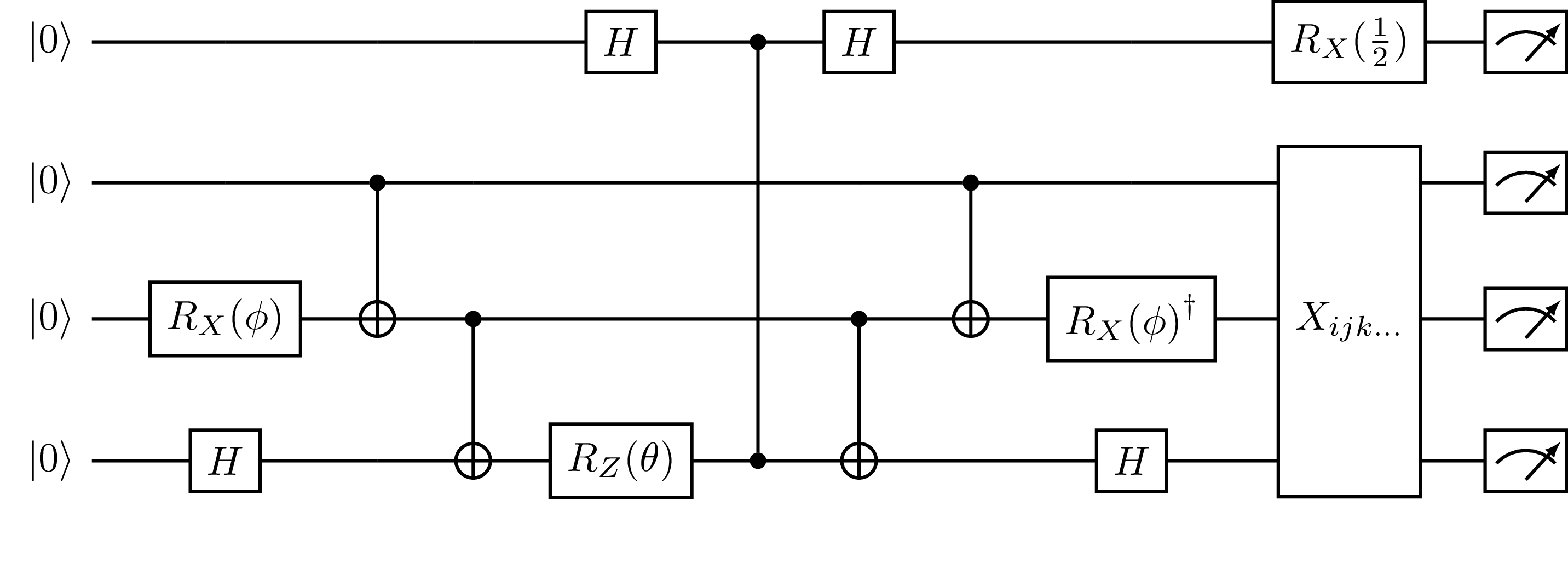
../../_images/hadamard_direct.png — Fig. 20 Measurement circuit generated by `HadamardTestDeriative` with `direct=True`, where \(X_{ijk\dots}\) is the set of gates required to measure a commuting set of Pauli terms in the Hamiltonian.

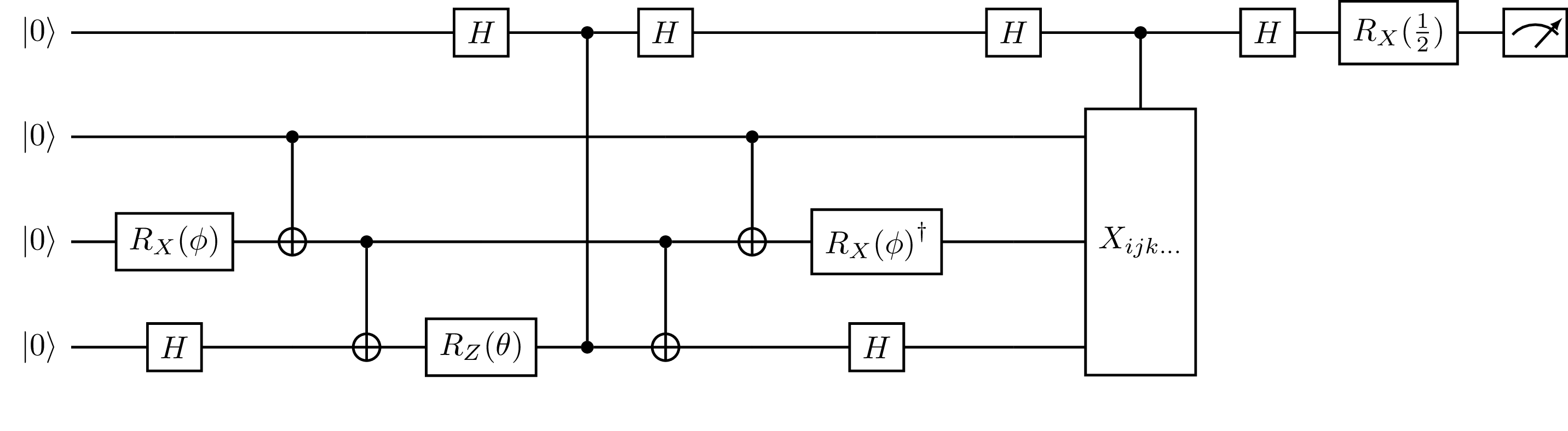
../../_images/hadamard_indirect.png — Fig. 21 Measurement circuit generated by `HadamardTestDerivative` with `direct=False`, where \(X_{ijk\dots}\) is the set of gates required to measure a commuting set of Pauli terms in the Hamiltonian.

HadamardTestDerivativeOverlap

The HadamardTestDerivativeOverlap is a shot-based protocol for computing elements of the metric tensor, based on refs [30, 34]. In terms of the regularized parameters, this is given by:

(56)\[\Braket{ \frac{\partial \psi}{\partial \theta_i} | \frac{\partial \psi}{\partial \theta_j} } = \sum_{kl} J_{ki} J_{lj} \Braket{ \frac{\partial \psi}{\partial \gamma_k} | \frac{\partial \psi}{\partial \gamma_l} }\]

The regularized derivative overlap is written as:

(57)\[\Braket{ \frac{\partial \psi}{\partial \gamma_k} | \frac{\partial \psi}{\partial \gamma_l} } = \Braket{\bar{0} | V_k(\gamma)^\dagger V_l(\gamma) | \bar{0} }\]

where \(V_i(\boldsymbol\gamma)\) is the i-th derivative of the regularized state preparation unitary:

(58)\[V_i(\boldsymbol\gamma) = U_n(\gamma_n)U_{n-1}(\gamma_{n-1})\dots U_i(\gamma_i) P_i \dots U_1(\gamma_1)U_0(\gamma_0)\]

This overlap may be evaluated with a modified Hadamard test. The Pauli strings injected by the derivatives are carefully applied to the state register, controlled on an ancilla qubit in a superposition state. For a calculation of the real part of the metric tensor (with \(k<l\)), this circuit is given by:

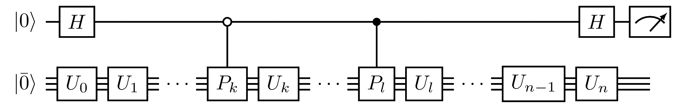
../../_images/metric_tensor.png — Fig. 22 Measurement circuit for the real part of the regularized derivative overlap: \(\text{Re}\Braket{\partial \psi / \partial \gamma_k | \partial \psi / \partial \gamma_l }\) generated by `HadamardTestDerivativeOverlap`.

As with a standard Hadamard test, the regularized derivative overlap is then given by

(59)\[\text{Re}\Braket{ \frac{\partial \psi}{\partial \gamma_k} | \frac{\partial \psi}{\partial \gamma_l} } = p(0) - p(1)\]

where \(p(b)\) is the probability of measuring the ancilla qubit in state \(b\in{0, 1}\). Equation (56) then provides the derivatives in terms of the original ansatz parameters. See a simple example below for a UCCSD ansatz:

from inquanto.express import get_system
from inquanto.ansatzes import FermionSpaceAnsatzUCCSD
from inquanto.protocols import HadamardTestDerivativeOverlap

_, fermion_space, hf_state = get_system("h2_sto3g.h5")
ansatz = FermionSpaceAnsatzUCCSD(
   fermion_space, hf_state
)
params = ansatz.state_symbols.construct_random()
symbols = ansatz.state_symbols.symbols
print(params)

protocol = HadamardTestDerivativeOverlap(AerBackend(), shots_per_circuit=5000)
protocol.build(
   parameters=params,
   state=ansatz,
   diff_symbols=(symbols[1], symbols[1])
)
protocol.run()
protocol.evaluate_derivative_overlap()

{d0: 0.9417154046806644, s0: -1.3965781047011498, s1: -0.6797144480784211}

{(s0, s0): 1.00000000000000}

We specify above that the HadamardTestDerivativeOverlap protocol should build circuits to calculate the (s0, s0) element of the metric tensor. The get_dataframe_derivative_overlap() method provides a breakdown of the circuits required for this calculation:

print(protocol.get_dataframe_derivative_overlap())

    symbols regularized symbols           prefactor  circuit index
(s0, s0)          (u14, u14)   0.250000000000000            NaN
(s0, s0)          (u14, u17)  -0.250000000000000            0.0
(s0, s0)          (u17, u14)  -0.250000000000000            0.0
(s0, s0)          (u17, u17)   0.250000000000000            NaN

which shows that only one circuit was required for this calculation. It also reveals that the ansatz regularization replaced two occurances of the symbol s0 with the parameters u14 and u17 in the 14th and 17th gates of the state preparation unitary respectively. The prefactor column shows the Jacobian product \(J_{ki}J_{lj}\). This protocol attempts to minimize the total number of circuits required by exploiting the fact that \(\text{Re}\Braket{\partial_k \psi| \partial_l \psi} = \text{Re}\Braket{\partial_l \psi| \partial_k \psi}\), and that diagonal elements are unity. Rows with a NaN circuit index mark these diagonal terms.